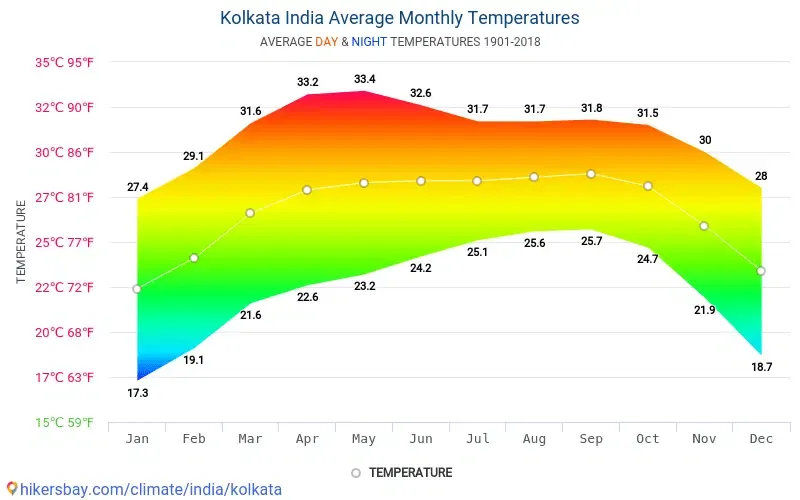
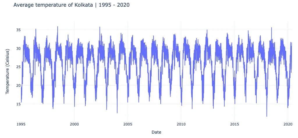
Average Monthly Temperature of Kolkata
In this article, I will explain the fundamentals of time series cross-validation using time series split and demonstrate how to implement this technique for time series forecasting in Python. Specifically, I will be focusing on predicting the average temperature in Kolkata from 2017 to 2020. This experiment will serve as the basis for my analysis, showcasing how time series split can be effectively used to improve forecasting accuracy.
Understanding Time Series Data: A Comprehensive Introduction
Time series data is a collection of observations or measurements recorded at a specific and evenly spaced time intervals. Each instance in the series represents the value of a variable at a particular moment, making the order of the data critical.
It is generally characterized by its sequential nature, which allows for the analysis of trends, patterns, and future predictions. This differs from other data types, where the order of data points may not matter and temporal relationships are not typically a focus.
Time series data are of two types:
- Continuous Time series data: Data Collected over time without any interruption.
Example: Hourly stock prices, person’s heart rate over time, etc. - Discrete Time series data: Data Collected and recorded at specific time intervals.
Example: Daily temperatures, quarterly GDP growth rate, etc.
Now, let’s dive into the code with an example to better understand time series cross-validation using time series split. We’ll learn the concepts as we go along.
Flow of Analysis :
- Importing the Required Libraries
- Loading the Data
- Feature Engineering and Data Cleaning
- Creating features for Time Series Forecasting
- Splitting the Data into Train and Test
- Cross-Validation in Time Series Forecasting
- Time Series Split and Its Implementation
- Model Building and Evaluation
1. Importing the Required Libraries
import pandas as pd
import numpy as np
import xgboost as xgb
import plotly.graph_objects as go
from plotly.subplots import make_subplots

from sklearn.model_selection import KFold,TimeSeriesSplit
from sklearn.metrics import mean_squared_error

import warnings
warnings.filterwarnings('ignore')
Here, I have imported all the necessary libraries for this analysis
2. Loading the Data
# reading the data
df = pd.read_csv(f'/kaggle/input/daily-temperature-of-major-cities/city_temperature.csv')
df.replace('Calcutta','Kolkata', inplace=True)
# selecting the city as Kolkata
df = df[df['City'] == 'Kolkata']
In this section, I’ve loaded the daily temperature data of major cities from a Kaggle dataset using pandas. I then filtered the data to focus specifically on the city of Kolkata. The dataset originally labeled the city as “Calcutta,” so I replaced “Calcutta” with “Kolkata” to reflect the current name before applying the filter.
https://www.kaggle.com/datasets/sudalairajkumar/daily-temperature-of-major-cities
3. Feature Engineering and Data Cleaning
# Creating a Date column for future reference
df['Date'] = df['Year'].astype(str) + '-' + df['Month'].astype(str) + '-' +df['Day'].astype(str)
df.set_index('Date', inplace = True)
df.index = pd.to_datetime(df.index)

fig = go.Figure()
fig.add_trace(go.Histogram(
    x=df['AvgTemperature'],nbinsx=500
))
fig.update_layout(
    title='Distribution of Average Temperature in Kolkata | 1995 - 2020',
    xaxis_title='Temperature (Fahrenheit)',
    yaxis_title='Frequency',
    template='plotly_white'
)
fig.show()
In this code, I create a Data column by combining the Year, Month, and Day columns, set it as the index, and convert it to date-time format for time series analysis. Then, I visualize the distribution of average temperatures in Kolkata from 1995 to 2020 using a histogram, to show the frequency of different temperature ranges and to look for any outliers in the data.
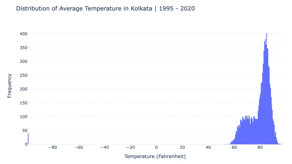
From the chart, it is clear that the average temperature in Kolkata typically ranges between 55 to 95 Fahrenheit. However, there are a few outliers around -99 Fahrenheit, which may indicate data errors or anomalies.
# dropping the wrong 'AvgTemperature' entries
df = df[df['AvgTemperature'] != -99]
# Converting AvgTemperature from Fahrenheit to Celsius
df['AvgTemperature'] = (df['AvgTemperature'] - 32) * 5 / 9
# dropping the Column State as it has all NaN Values
df.drop(columns = ['State'], inplace= True)
In this section, I removed rows with incorrect temperatures (-99), converted temperatures from Fahrenheit to Celsius, and dropped the State column due to Nan values.
Now, this is the final time series dataset, prepared and cleaned for analysis.
4. Creating features for Time Series Forecasting
# Creating features
df['dayofweek'] = df.index.dayofweek
df['quarter'] = df.index.quarter
df['dayofyear'] = df.index.dayofyear
df['weekofyear'] = df.index.isocalendar().week
df['SMA_90'] = df['AvgTemperature'].rolling(90).mean()
df['SMA_60'] = df['AvgTemperature'].rolling(60).mean()
df['SMA_30'] = df['AvgTemperature'].rolling(30).mean()
df['Yesterday_Temperature'] = (df.index - pd.Timedelta('1 days')).map(df['AvgTemperature'].to_dict())
df.dropna(inplace = True)
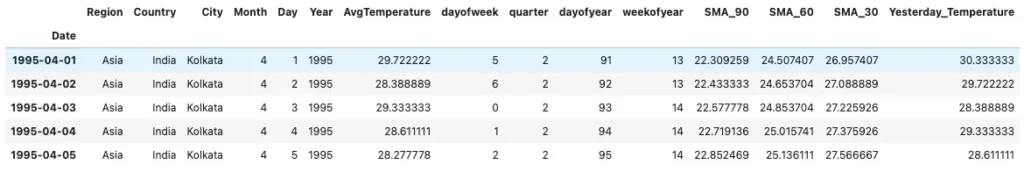
df.head()In this section, I created features such as day of the week, quarter, day of the year, week of the year, rolling averages, and yesterday’s temperature. I then removed rows with missing values, and here is a glimpse of the data:
5. Splitting the Data into Train and Test
# Splitting the data for train (including validation) and test

train = df.loc[:'2017-01-01']
# Keeping a gap of 4 months to avoid lookahead through the SMA 90
test = df.loc['2017-04-01':]

fig = go.Figure()
fig.add_trace(go.Scatter(
    x=train.index,y=train['AvgTemperature'],mode='lines',name='Training Set'
))
fig.add_trace(go.Scatter(
    x=test.index,y=test['AvgTemperature'],mode='lines',name='Test Set'
))
fig.add_shape(
    type="line",x0='2017-04-01',y0=9,x1='2017-04-01',y1=max(train['AvgTemperature'].max(), test['AvgTemperature'].max()),
    line=dict(color="green", width=2, dash="dash")
)
fig.update_layout(
    title='Data Split into Train and Test ',
    xaxis_title='Date',
    yaxis_title='Temperature (Celsius)',
    template='plotly_white',
    legend=dict(orientation='h',yanchor='bottom',y=1.02,xanchor='right',x=1),
)
fig.show()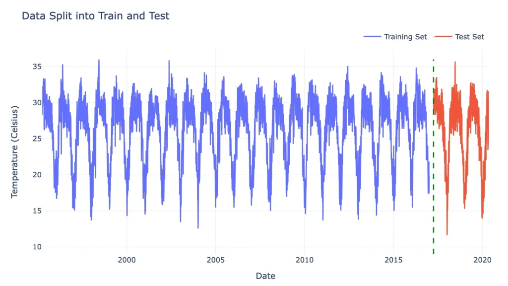
In this section, I split the data into training (before 2017) and test (2017 and after) sets.
6. Cross-Validation in Time Series Forecasting
Cross-validation in time series forecasting is crucial because it helps ensure that the model’s performances is robust and generalizes well to unseen data. Unlike in standard machine learning, where data points are randomly split into training and test sets, time series data must maintain it’s temporal order.
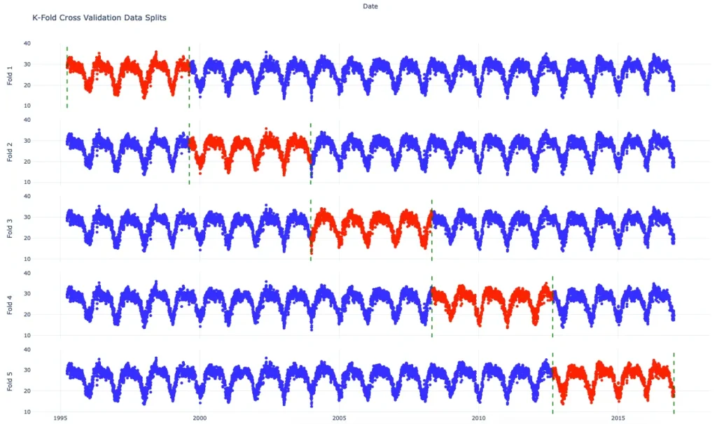
Traditional cross-validation methods, such as k-fold cross-validation, are unsuitable for time series data because they randomly divide the data into training and test sets, which disrupts the chronological sequence.
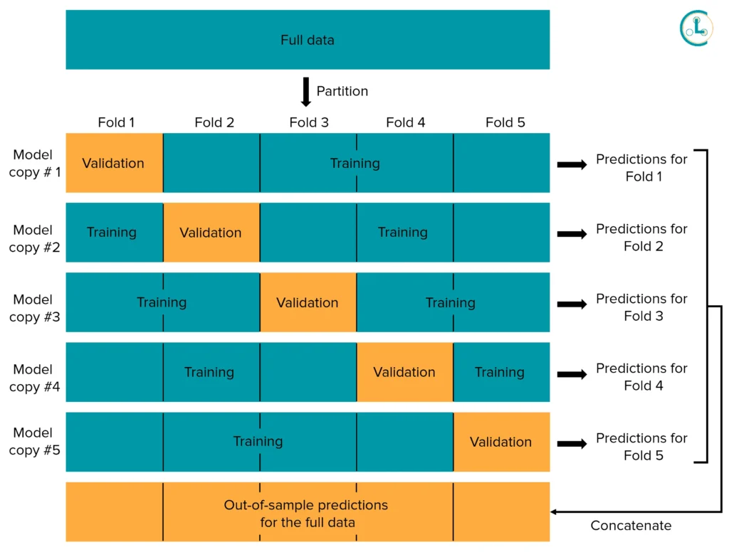
Working of K-Fold Cross Validation Technique. Source : Cleanlab
This is problematic for the following reasons:
- Disrupts Temporal Sequence: These methods can mix past and future observations, violating the natural order of time. Time series data relies on the sequence of events, and random splits can lead to situations where future data influences past predictions.
- Breaks Time-Dependent Patterns: Time series data often shows trends, seasonal effects, and other time-based patterns. Randomly shuffling the data prevents the model from accurately learning and capturing these time-dependent relationships.
- Unrealistic Test Conditions: Traditional cross-validation might test the model on data that isn’t sequentially aligned with the training set, creating scenarios that don’t reflect how forecasting works in practice.
Maintaining the temporal order of data is vital for several reasons:
- Accurate Forecasting: Models need to be trained on data in its natural sequence to effectively learn how past events influence future outcomes.
- Realistic Model Evaluation: Testing the model on data that follows the training set reflects real-world forecasting scenarios where predictions are made based on historical data.
- Pattern Recognition: Keeping the order helps capture trends and seasonal patterns that are crucial for making accurate forecasts.
Using time series-specific cross-validation methods, like time series split, ensures that data is handled sequentially, preserving the natural order and dependencies essential for effective forecasting.
7. Time Series Split and Its Implementation
Introduction :
Time Series Split is a cross-validation method tailored for time series data, ensuring that the chronological order of observations is maintained. Unlike traditional cross-validation techniques that randomly split the data, time series split preserves the sequence of the data, reflecting real-world forecasting scenarios.
Below is the working principle of time series split:
- Sequential Division: Data is split into training and validation sets in a sequential manner. Each iteration involves creating a training set that grows over time and a validation set that follows it.
- Expanding Window: The training set expands with each iteration while the validation set moves forward in time. For example, you might start by training on the first 12 months and validating on the next month, then train on the first 13 months and validate on the subsequent month, and so on.
- Rolling Window: Another approach is the rolling window method, where both the training and validation sets shift forward. For instance, you might train on months 1–12 and validate on months 13–14, then train on months 2–13 and validate on months 14–15, and continue this process.
Advantages:
- Preserves Time Order: Maintains the natural sequence of data, ensuring that training data precedes validation data, which mirrors actual forecasting conditions.
- Captures Temporal Patterns: Allows models to learn and validate on time-dependent trends and patterns effectively.
- Multiple Assessments: Provides several training and validation pairs, offering a thorough evaluation of model performance across different periods.
Implementation :
time_series_split = TimeSeriesSplit(n_splits=5, test_size=365*2, gap=90)

fig = make_subplots(rows=5, cols=1, shared_xaxes=True, vertical_spacing=0.03)
fold = 0
for train_idx, val_idx in time_series_split.split(train):
    train_cv = train.iloc[train_idx]
    val_cv = train.iloc[val_idx]

    fig.add_trace(go.Scatter(
        x=train.index,y=train_cv['AvgTemperature'],mode='markers',line=dict(color='blue'),
        name=f'Training Set Fold {fold + 1}',),row=fold + 1, col=1)

    fig.add_trace(go.Scatter(
        x=val_cv.index,y=val_cv['AvgTemperature'],mode='markers',line=dict(color='red'),
        name=f'Test Set Fold {fold + 1}',), row=fold + 1, col=1)

    fig.add_shape(type="line",
                  x0=val_cv.index.min(),y0=9,
                  x1=val_cv.index.min(),y1=40,
                  xref='x', yref=f'y{fold + 1}',
                  line=dict(color="green", width=2, dash="dash"),row=fold + 1, col=1
    )
    fig.add_shape(type="line",
                  x0=val_cv.index.max(),y0=9,
                  x1=val_cv.index.max(),y1=40,
                  xref='x', yref=f'y{fold + 1}',
                  line=dict(color="green", width=2, dash="dash"),row=fold + 1, col=1
    )
    fig.update_yaxes(title_text=f'Fold {fold + 1}', row=fold + 1, col=1)
    fold += 1

fig.update_layout(
    height=1000,
    title_text='Time Series Split Cross Validation Data Splits',
    xaxis=dict(title='Date'),
    showlegend=False,
    template='plotly_white'
)
fig.show()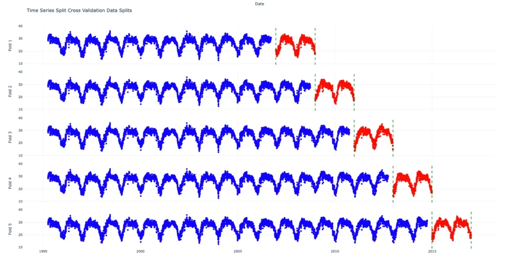
In this section, I implemented a Time Series Split cross-validation with 5 splits, each including a 2-year test set and a 90-day gap. The plot shows how the data is divided into training and validation sets for each fold, with training data in blue and validation data in red. Green dashed lines indicate the boundaries of the validation periods.
8. Model Building and Evaluation
# Model training using Time Series Split
time_series_split = TimeSeriesSplit(n_splits=5, test_size=365*2, gap=20)
fold = 0
best_params = {
    'learning_rate': 0.05,
    'n_estimators': 1000,
    'max_depth': 6,
    'early_stopping_rounds': 50,
    'subsample': 0.8,
    'colsample_bytree': 0.8,
    'gamma': 0.1,
    'min_child_weight': 5,
    'reg_alpha': 0.1,
    'reg_lambda': 1,
    'objective': 'reg:squarederror',
    'random_state': 42,
    'booster': 'gbtree'
}

for train_idx, val_idx in time_series_split.split(train):
    train_cv = df.iloc[train_idx]
    val_cv = df.iloc[val_idx]

    X_FEATURES = ['Month', 'Day', 'Year', 'dayofweek', 'quarter', 'dayofyear', 'weekofyear', 'SMA_90', 'SMA_60',
       'SMA_30', 'Yesterday_Temperature']
    TARGET = 'AvgTemperature'

    X_train = train[X_FEATURES]
    y_train = train[TARGET]

    X_val = val_cv[X_FEATURES]
    y_val = val_cv[TARGET]

    model = xgb.XGBRegressor(**best_params)
    model.fit(X_train, y_train,eval_set=[(X_train, y_train), (X_val, y_val)],verbose=100)
In this section, I trained the model using Time Series Split cross-validation with 5 folds. For each fold, I used the best hyper parameters for the XGBoost regressor to train on the training data and evaluate on the validation data. Features include date-related variables and rolling averages, while the target is AvgTemperature.
Model Evaluation
# Seperating the test dataset
X_test = test[X_FEATURES]
y_test = test[TARGET]

X_train = train[X_FEATURES]
y_train = train[TARGET]

# Prediction Using the model
y_pred_test = model.predict(X_test)
y_pred_train = model.predict(X_train)

train["Predicted_Avg_Temp"] = y_pred_train
test["Predicted_Avg_Temp"] = y_pred_test

# Evaluating the model
print(f'MSE on the Train Set : {mean_squared_error(y_train, y_pred_train)}')
print(f'MSE on the Train Set : {mean_squared_error(y_test, y_pred_test)}')
In this section, I separated the test dataset and made predictions using the trained model. I evaluated the model by calculating the Mean Squared Error (MSE) for both the training and test sets, which were 0.360 on the train set and 1.776 on the test set.
fig = go.Figure()

fig.add_trace(go.Scatter(
    x=test.index,y=test['AvgTemperature'],mode='lines',name='Actual Test'
))
fig.add_trace(go.Scatter(
    x=test.index,y=test['Predicted_Avg_Temp'],mode='lines',name='Predicted Test'
))

fig.update_layout(
    title='Comparison of Actual vs Predicted Values | Test',
    xaxis_title='Date',
    yaxis_title='Temperature (Celsius)',
    template='plotly_white',
    legend=dict(orientation='h',yanchor='bottom',y=1.02,xanchor='right',x=1)
)
fig.show()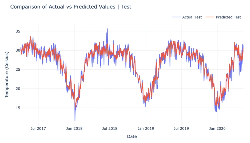
In this section, I created a plot comparing the actual and predicted temperatures for the test set. The graph displays actual temperatures in one line and predicted temperatures in another, allowing for visual comparison.
Summary and Key Takeaways:
Model Performance:
- The model demonstrated strong predictive capability, achieving a Mean Squared Error (MSE) of 0.360 on the training set and 1.776 on the test set. This indicates that the model generalized well to unseen data, though there was a slight increase in error when applied to the test set, which is expected in time series forecasting.
Trend and Seasonality Capture:
- The model effectively captured both the underlying trend and seasonal patterns present in the data. This is crucial for time series forecasting, as it allows the model to make more accurate predictions over time.
Time Series Split Effectiveness:
- Utilizing time series split for cross-validation ensured that the model’s performance was evaluated in a way that respects the temporal sequence of the data. This approach validated the model’s ability to predict future data based on past trends, increasing confidence in its forecasting power.
Visualization Insights:
- The visual comparison between predicted and actual data highlighted the model’s accuracy in tracking the actual values over time. Minor discrepancies were observed but were within an acceptable range, affirming the model’s robustness.
Practical Implications:
- The model’s ability to capture trends and seasonality makes it a valuable tool for forecasting in real-world applications, such as financial planning, inventory management, or demand forecasting.
Areas for Future Improvement:
- While the model performed well, exploring advanced techniques or incorporating additional features could further reduce the error on the test set. Future work could also involve experimenting with different models or fine-tuning hyper parameters to enhance performance.
Thank you for reading! I hope this article provided valuable insights into time series cross-validation and forecasting.
Here is the notebook that I used for this analysis:
https://www.kaggle.com/code/subhasishsaha/time-series-forecasting-using-time-series-split
Please check it out for more details and a better understanding.
You can also connect with me on