
In this post I will talk about the Masked Autoencoder for Distribution Estimation MADE which was covered in a paper in 2015 as linked above. I will follow the implementation from University of Berkeley’s Deep Unsupervised Learning course which can be found here.
Complete code is stored in accompanying github repository.
This post is broken into following sections:
- Introduction
- PyTorch Implementation
- Running Experiments
1. Introduction
Autoencoders are a neural network which is used to learn the data representation in an efficient and unsupervised manner. e.g. if we give a set of cat images to an autoencoder, it should then be able to generate new cat images i.e. synthetic images which look like cats. While there a lot of different types of autoencoders, the focus of this article will be Masked Autoencoders for (Data) Distribution Estimation (MADE).
In mathematical terms we want to estimate [latex]p_{data}[/latex] from the samples
[latex]
\begin{align*}
\boldsymbol{x^{(1)}, x^{(2)}, …, x^{(n)} \sim p_{data}(x)}
\end{align*}
[/latex]
Suppose each sample [latex]\boldsymbol{x}[/latex] is [latex]k[/latex] dimensional. In other words [latex] \boldsymbol{x} [/latex] is a vector with [latex] k [/latex] elements:
[latex]
\begin{align*}
\boldsymbol{x} = [x_1, x_2, …., x_k]
\end{align*}
[/latex]
Let us say we want to estimate the probability of seeing the sample [latex]\boldsymbol{x^{(n)}}[/latex]. We can factorize the probability of the sample into its [latex] k [/latex] – dimensions using conditional probability and product rule as shown below:
[latex]
\begin{align*}
p(\boldsymbol{x})=p(x_1, x_2, …., x_k)
\end{align*}
[/latex]
factorizing the joint distribution into product of conditional distribution:
[latex]
\begin{align*}
p(\boldsymbol{x})=p(x_1).p(x_2 | x_1).p(x_3|x_1, x_2)…p(x_k|x_1, x_2,..,x_{k-1}) \text{…..(1)}
\end{align*}
[/latex]
In masked autoencoder, we design a neural network which takes the [latex]k[/latex] dimensional input [latex]\boldsymbol{x}[/latex] and produces another [latex]k[/latex] dimensional output, the [latex] k [/latex] conditional distributions as decomposed in equation (1) above. MADE is a neural network with [latex] k [/latex] inputs and [latex] k [/latex] outputs with some constraints specified as per equation (1), i.e. the output [latex] \hat{p}(x*l) [/latex] depends only on the values [latex] x_1, …., x*{l-1} [/latex] i.e. inputs before it. In other words, we enforce a connection constraint such that input [latex] x*l [/latex] can connect only to the outputs [latex] \hat{x}*{l+1} [/latex] onwards.
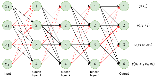
Figure 1: Sample MADE autoencoder
In figure 1, a fully connected neural network with 3 hidden layers is shown. The existing connections are shown in black arrows and missing connections are shown in red dashed arrows. If you follow all the inputs leading to a specific output node, you will notice that for output node [latex] p(x*l) [/latex] only inputs from [latex] x_1 [/latex] to [latex] x*{l-1} [/latex] are connected to it. Which enforces the auto-regressor property that [latex] p(x_l) [/latex] only depends on the prior dimensions of the input [latex] \boldsymbol{x} [/latex]. The red arrows show the connections that have been masked out from a fully connected layer and hence the name Masked autoencoder.
1.1 Two types of mask
Once again notice the connections between input layer and first hidden layer and look at the node 3 in the hidden layer. You will notice that node 3 is connected to only the previous inputs less than 3 i.e. node 3 of hidden layer is connected to only [latex] x_1 [/latex] and [latex] x_2 [/latex]. In other words, node [latex] l [/latex] in hidden layer 1 is connected to inputs [latex] x_i[/latex], i < l. We call this type 1 mask.
If you notice other connections e.g. hidden layer 1 to hidden layer 2 or hidden layer 2 to hidden layer 3 or the final connections to output layer, you will notice that here node [latex] l [/latex] in a layer is connected to all the nodes in previous layer upto and including node [latex] l [/latex]. We call this type 2 mask.
In order to ensure that [latex] l^{th} [/latex] output depends only on inputs [latex] x*1, x_2, …, x*{l-1} [/latex], thereby having auto-regressor property, we need atleast one type 1 mask layer while all other layers could be of type 2 mask. And position of the type 1 mask could be any of the layers. It need not be first one like we showed in the figure 1 above. The paper used type 1 mask at the last set of connections i.e. last hidden layer to output connections. The paper calls the type 1 mask [latex] M^V [/latex] and type 2 mask as [latex] M^W [/latex].
1.2 Numbering the nodes in hidden layer
If you look at figure 1, you will notice that the number of nodes in each hidden layer is same as the number of input nodes in our diagram. That was just to simplify the illustration. The way paper goes about this is that:
- each hidden layer can have any size i.e. any number of nodes
- suppose the input has a dimension [latex]d[/latex]. Each node in a hidden layer is assigned a number between [latex] 1 [/latex] to [latex] d-1 [/latex] i.e. kth hidden unit in a specific hidden layer is given a number denoted by 0 < [latex]m(k)[/latex] < d-1.
1.3 Input Ordering
The paper also suggested the flexibility to order the inputs so that joint probability [latex] p(\boldsymbol{x}) [/latex] could be broken into any specific order. Consider a 3-dimensional input [latex] \boldsymbol{x} = [x_1, x_2, x_3] [/latex]. We could break this joint distribution in any order of input dimensions such as:
[latex]
p(\boldsymbol{x}) = p(x_1) . p(x_2 | x_1) , p(x_3 | x_1, x_2) \\
p(\boldsymbol{x}) = p(x_2) . p(x_1 | x_2) , p(x_3 | x_2, x_1) \\
p(\boldsymbol{x}) = p(x_3) . p(x_1 | x_2) , p(x_2 | x_3, x_1) \\
p(\boldsymbol{x}) = p(x_1) . p(x_3 | x_1) , p(x_2 | x_1, x_2) \\
p(\boldsymbol{x}) = p(x_2) . p(x_3 | x_2) , p(x_1 | x_2, x_3) \\
p(\boldsymbol{x}) = p(x_3) . p(x_2 | x_3) , p(x_1 | x_3, x_2) \\
[/latex]
The paper used input ordering to train the model to predict all possible combinations of joint probability breakdown.
Let us explain all the concepts with the help of an example. We show below the sample Masked autoencoder from figure 1 of the MADE paper.
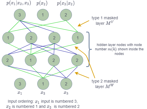
Figure 2: MADE autoencoder with full details (ref: figure 1 of the paper)
In the figure you can see that input layer ordering is shown as [3, 1, 2]. The dimension of input is [latex] d=3 [/latex]. The mask from input to 1st hidden layer is of type 2 ([latex] M^W [/latex]) in which the node [latex] k [/latex] from lower layer with node numbered [latex] m(k) [/latex] is connected to all the nodes in upper layer with nodes numbered [latex] m(k) [/latex] to [latex] d [/latex]. The green arrows show that node 1 from lower layer is connected to all the nodes numbered from 1 to 3 in upper layer. The blue arrows show the similar connected for node numbered 2 in lower layer.
The connections from 1st hidden layer to 2nd hidden layer also follow the same logic with mask [latex] M^W [/latex].
However, the connection from last hidden layer to output layer follow mask of type [latex] M^V [/latex] in which node numbered [latex] m(k) [/latex] from lower layer is connected to nodes in upper layer numbered [latex] m(k)+1 [/latex] to [latex] d [/latex].
From the figure you can see that output node numbered 1 has no connection and it produces the probability distribution [latex] p(x_2) [/latex]. Similarly, the node numbered 2 has only green connections i.e. only getting value from input node numbered 1. The node numbered 3 has green and blue connections which trace back to input nodes numbered 1 and 2. The input node numbered 3 does not feed to anything.
1.4 How do we train a model
In unsupervised setup when we are trying to teach the model to learn the data distribution, we feed unlabelled samples [latex] \boldsymbol{x^{(1)}, x^{(2)}, …, x^{(n)}} [/latex] and we adjust the neural network parameters denoted as [latex] \theta [/latex] to increase the probability of observing these samples e.g.:
[latex]
\begin{align*}
p_{\theta}(\boldsymbol{x}) = p(x_1).p(x_2|x_1)….p(x_k|x_1,…x_{k-1})
\end{align*}
[/latex]
Dropping the conditional variables in the factors above to simplify the notation, we get:
[latex]
\begin{align*}
p_{\theta}(\boldsymbol{x}) = p(x_1).p(x_2)….p(x_k)
\end{align*}
[/latex]
We need to maximize the probability [latex] p(\boldsymbol{x}) [/latex]. As [latex] log [/latex] is a monotonically increasing function, we could also maximize the log of probability i.e. [latex] \log {p(\boldsymbol{x})} [/latex]. This is known as maximizing the log likelihood of the probability. Since all deep learning libraries have minimizer instead of maximizer, we turn log likelihood maximization into a minimization by putting a -ve sign before the log. This is known as negative log likelihood (NLL).
[latex]
\begin{align*}
NLL = – \log{p_{\theta}(\boldsymbol{x})}
\end{align*}
[/latex]
Rewriting,
[latex]
\begin{align*}
NLL = – \sum_{k=1}^d \log{p_{\theta}(x_k)}
\end{align*}
[/latex]
Let us consider situation where each input dimension [latex] x_k [/latex] can take only two values {0, 1} i.e. a black and while pixel with 0 indicating a black pixel and 1 indicating a white pixel. Let us say the input [latex] \boldsymbol{x} [/latex] is the vector of individual pixels of a black/white image. If the image is 20×20 pixels i.e. d= 400 pixels, each of value either 0 or 1. We run this image through the MADE neural network as shown in figure 2 above. The output layer produces 400x2 values, two values for each pixel denoting the log probability that a pixel is either 0 or 1.
[latex]
\begin{align*}
\begin{pmatrix}
-\log{p(x_1=0)} & -\log{p(x_1=1)} \\
\cdot & \cdot \\
-\log{p(x_k=0)} & -\log{p(x_k=1)} \\
\cdot & \cdot \\
\cdot & \cdot \\
-\log{p(x_d=0)} & -\log{p(x_d=1)} \\
\end{pmatrix}
\end{align*}
[/latex]
Based on the actual input pixel value [latex] x_k [/latex] being either 0 or 1, we pick the corresponding [latex]-\log{p(x_k=0)} [/latex] or [latex]-\log{p(x_k=1)} [/latex]. We do this for each of the 400 pixels, sum them up and try to adjust the network parameters [latex] \theta [/latex] so that the sum (i.e. NLL) is minimized.
NLL is also known as cross-entropy loss and is available as torch.nn.functional.cross_entropy(input, target)
Let us say we have a batch of 400 pixel black/white images and let the batch size be b. In this case the training batch is of shape (bx400). The training batch is what is fed as target in above function.
We one-hot encode the data which changes the shape to (bx400x2) for the black and white image case where each pixel can only be 0 or 1. This one hot encoded vector is fed into the neural network producing the log probabilities of each pixel being 0 or 1. The output is also of the same shape (bx400x2). This output/prediction is fed into cross_entropy function as parameter input.
The optimizer in PyTorch minimizes the value of cross_entropy loss or in other words increases the likelihood of the training input.
We run the system them multiple batches of input images. At the end of training, the model has learnt the representation of the pixel value distribution of input images. Now this model can be used to generate the synthetic images as explained in next section.
1.4 Generating a synthetic sample image
Look back at figure 2. After the model has been trained, we will look at node 1 value i.e. [latex] p(x_2) [/latex] and use this distribution to generate the pixel [latex] x_2 [/latex] e.g. using a Bernoulli distribution in case of black/white image with no grey scales. The pixel value [latex] x_2 [/latex] generated is fed again into the model to get an estimate of [latex] p(x_3 | x_2) [/latex]. This probability is used to generate the pixel [latex] x_3 [/latex]. The pixel values [latex] x_2 [/latex] and [latex] x_3 [/latex] are once more fed into the trained network to produce the estimate [latex] p(x_1\|…) [/latex]. Like before a value is sampled from probability estimate to generate the pixel [latex] x_1 [/latex].
You can see that image generation is a serial process, we need to generate one pixel at a time. For a 20×20 image, we will need 400 passes through the network to produce the image.
This covers all the theoretical explanations. In next section we will dive deep into the PyTorch implementation.
2. PyTorch Implementation
Having covered the theory, we will now look at implementation. Let us first look at the data we will use for training the model. We will use Shapes dataset which is a set of images of 2D geometric shapes. We will use a scaled down version of the dataset comprising of 10479 images of shape 20x20x1 i.e. 20×20 pixel images with single greyscale images. We will convert the greyscale to {0,1} discreet valued dataset. The test set will have 4491 images of same shape.
2.1 Exploring training data
Let us explore the data. We will use torchvision.utils.make_grid function to sample 100 images from train_data and plot the same in 10×10 grid. Please note that train_data and test_data have a shape 20x20x1 (HxWxC with C, the number of channels=1). However, PyTorch expects the data in channel_first format. You will see we transposing the data from (H, W, C) to (C, H, W) multiple times in the code as matpotlib expects the data to have a shape of (H, W, C) while PyTorch expects the same to be of shape (C, H, W).
There are two utility functions, load_data to load the dataset form pickled file and show_samples to show the sampled images. We will not go into the implementation of these functions. However, readers may find it interesting to go over the same as an extra.
The code to load and display the samples is:
# load data

train_data, test_data = load_data()
name = "Shapes dataset"
print (f'Train Shape: {train_data.shape}')
print (f'Test Shape: {test_data.shape}')

# sample 100 images from train data

idxs = np.random.choice(len(train_data), replace=False, size=(100,))
images = train_data[idxs] \* 255

# show 100 samples in a 10x10 grid

show_samples(images, title=f'"{name}" Samples')
A sample of images is shown below:
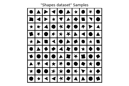
Figure 3: Sample data from Shapes dataset
2.2 Generic Training loop
Next we look at a generic training loop over a given number of epochs. The function train_epochs gets a model as the input. In our case it will be a MADE model which we will talk about in upcoming paragraphs. It also gets a train_loader, test_loader which are of type torch.utils.data.DataLoader. DataLoader provides a python iterable over a dataset. The function also gets a dictionary of additional parameters such as _learningrate, _noepochs and gradient clipping values. The function train_rpochs returns an array of train_losses and test_losses where test_losses are one loss value on test_data at the end of each epoch and train_losses are train losses for each batch giving up a more fine grained progress of train_loss during the entire training phase.
def train_epochs(model, train_loader, test_loader, train_args):
epochs, lr = train_args['epochs'], train_args['lr']
grad_clip = train_args.get('grad_clip', None)
optimizer = optim.Adam(model.parameters(), lr=lr)

    train_losses = []
    test_losses = [eval_loss(model, test_loader)]
    for epoch in range(epochs):
        model.train()
        train_losses.extend(train(model, train_loader, optimizer, epoch, grad_clip))
        test_loss = eval_loss(model, test_loader)
        test_losses.append(test_loss)
        print(f'Epoch {epoch}, Test loss {test_loss:.4f}')

    return train_losses, test_losses
Function train_epochs uses two other functions. Function train runs a single epoch of training returning the array of training losses per batch in a single epoch. eval_loss runs the model trained so far on the test_data to produce the average test loss for the test_data. PLease note that we use with torch.no_grad(): to make sure that no gradient values are accumulated while going through the test_data valuation.
def train(model, train_loader, optimizer, epoch, grad_clip=None):
model.train()

    train_losses = []
    for x in train_loader:
        x = x.cuda().contiguous()
        loss = model.loss(x)
        optimizer.zero_grad()
        loss.backward()
        if grad_clip:
            torch.nn.utils.clip_grad_norm_(model.parameters(), grad_clip)
        optimizer.step()
        train_losses.append(loss.item())
    return train_losses

def eval_loss(model, data_loader):
model.eval()
total_loss = 0
with torch.no_grad():
for x in data_loader:
x = x.cuda().contiguous()
loss = model.loss(x)
total_loss += loss \* x.shape[0]
avg_loss = total_loss / len(data_loader.dataset)

    return avg_loss.item()
Now we will look into building the MADE model. For a single layer of masked layer as shown in figure 2, we will sub class the torch LinearLayer (nn.Linear) and apply a specific mask to switch off the specific connections. The mask will be created outside and will be set using set_mask function. We use torch‘s register_buffer to create a buffer named mask to create the storage space for the mask. This mask is used in the forward. We multiply the self.weights that we get from nn.Linear super class with mask to switch off the specific connections from input nodes to the output nodes. The code is shown below:
class MaskedLinear(nn.Linear):
def **init**(self, in_features, out_features, bias=True):
super().**init**(in_features, out_features, bias)
self.register_buffer('mask', torch.ones(out_features, in_features))

    def set_mask(self, mask):
        self.mask.data.copy_(torch.from_numpy(mask.astype(np.uint8).T))

    def forward(self, input):
        return F.linear(input, self.mask * self.weight, self.bias)
2.3 MADE in PyTorch
Next, we will define the complete MADE model which is created by extending PyTorch’s nn.Module class. We will use a network with 2 hidden layers each of size 512 nodes. Let us first look at the __init__ function. Here we get the shape of the input input_shape. IN our current example it is (1x20x20) with channel first style of image representation. We also get d the dimension of each pixel value i.e. the range of possible values each pixel can take. This is 2 in our current case as each pixel can have only two possible values {0,1}. We also get an array hidden_sizes with the number nodes in hidden layers. Finally we get ordering which specifies the order in which we want the pixel values to be dependent on each other as explained in section 1.3 above. In case no ordering is provided, we create one on the fly with np.arange(self.nin). We store all these values in instance variables. The total number of inputs self.nin is equal to the product of input_shape. With our current example having images of shape (1x20x20), we have 400 inputs. d is 2 as explained above. Accordingly, the number of output nodes self.nout is 400×2=800.
class MADE(nn.Module):
def **init**(self, input_shape, d, hidden_size=[512, 512, 512],
ordering=None):
super().**init**()
self.input_shape = input_shape
self.nin = np.prod(input_shape)
self.nout = self.nin \* d
self.d = d
self.hidden_sizes = hidden_size
self.ordering = np.arange(self.nin) if ordering is None else ordering

      # define a simple MLP neural net
      self.net = []
      hs = [self.nin] + self.hidden_sizes + [self.nout]
      for h0, h1 in zip(hs, hs[1:]):
          self.net.extend([
            MaskedLinear(h0, h1),
            nn.ReLU(),
          ])
      self.net.pop()  # pop the last ReLU for the output layer
      self.net = nn.Sequential(*self.net)

      self.m = {}
      self.create_mask()  # builds the initial self.m connectivity
We create a simple nn.Sequential based neural network. We also create the masks by calling function self.create_mask(). This function is what differentiates MADE from a regular fully connected layers based network. The function creates the masks to allow/block connections as shown in figure 2. In line 2 of the code as shown below, we store in L the number of hidden layers. The variable self.m holds the number [latex] m(k) [/latex] attached to each node in each layer. Input layer will have the provided ordering as shown in the lower layer in figure 2. In case there is no ordering provided, we initialize the ordering with values so that pixels are numbered in a raster scan order i.e. go across the pixels in a row first and then move to next row, starting from top left of the image and move over to bottom right pixel, one row at a time. self.m[-1] denotes the input layer.
For each of the hidden layer for l in range(L):, we assign a number which is >= the minimum node value from lower layer all the way till the d-1 as explained in 1.2 i.e. mask [latex] M^W [/latex]. ALso please note that since we start the numbering from 0 instead of 1 as shown in paper, the input nodes will be numbered from 0 to d-1 i.e. 399 in our case. The first hidden layer will have nodes numbered form 0, the minimum number in input node to d-2 i.e. 398. The code carrying out this assignment of numbers to nodes in all hidden layers is given in line numbers 6 to 8. The next hidden layer will have nodes numbered from the minimum number across the previous layer nodes and will go upto d-2.
The output nodes will be numbered same as the numbers assigned to the input layer. Also the size of output layer is same as that of input layer multiplied by self.d, the number of discrete values the input can take. self.d is 2 in our case as pixels can take only two values {0, 1}.
def create_mask(self):
L = len(self.hidden_sizes)

    # sample the order of the inputs and the connectivity of all neurons
    self.m[-1] = self.ordering
    for l in range(L):
        self.m[l] = np.random.randint(self.m[l - 1].min(),
                                        self.nin - 1, size=self.hidden_sizes[l])

    # construct the mask matrices
    masks = [self.m[l - 1][:, None] <= self.m[l][None, :] for l in range(L)]
    masks.append(self.m[L - 1][:, None] < self.m[-1][None, :])

    masks[-1] = np.repeat(masks[-1], self.d, axis=1)

    # set the masks in all MaskedLinear layers
    layers = [l for l in self.net.modules() if isinstance(l, MaskedLinear)]
    for l, m in zip(layers, masks):
        l.set_mask(m)
Lines 10 to 14 create the masks. In line 11, we create the type 2 masks [latex] M^W [/latex] connecting input to 1st hidden layer and the subsequent layer connections till the last hidden layer.
The last hidden layer to output layer is connected via [latex] M^V [/latex] type of mask. Please note that output layer has self.d output nodes for each input node so that for each pixel we can predict the multinomial probability distribution of each pixel across all possible self.d values. Accordingly, we first create a mask in line 14 and then replicate it self.d times in line 14. Lines 17 to 19 set the masks created above in each MaskedLinear layer.
Next, the forward function is pretty simple. We flatten the input from shape (batch_size, 1, 20, 20) to shape (batch_size, self.nin), pass it through the MaskedLinear layers stored in self.net, also converting the output shape (batch_size, self.nout) to (batch_size, self.nin, self.d). We then swap the last two axes to reshape the output to (batch_size, self.d, self.nin). Finally we shape it further to (batch_size, self.d, 1, 20, 20).
def forward(self, x):
batch_size = x.shape[0]
x = x.float()
x = x.view(batch_size, self.nin)

        logits = self.net(x).view(batch_size, self.nin, self.d)
        return logits.permute(0, 2, 1).contiguous().view(batch_size, self.d, *self.input_shape)
Calculation of loss is very simple. We take the input, pass it through the forward function and then calculate the cross_entropy between the predicted outputs and the inputs. This gives us the NLL for the data. The loss is then fed to PyTorch optimizer to reduce the NLL or increase the occurrence probability of samples.
def loss(self, x):
return F.cross_entropy(self(x), x.long())
Finally we have sample function to generate samples from the trained model. Please note in order to generate the output pixels, we have to go over all the pixels in the order as specified in ordering, generating one pixel at a time as well as feeding all the previous pixels as inputs. We use torch.no_grad to avoid accumulating the gradients. Finally before returning the sample images we move them from GPU to CPU.
def sample(self, n):
samples = torch.zeros(n, self.nin).cuda()
self.inv_ordering = {x: i for i, x in enumerate(self.ordering)}

    with torch.no_grad():
        for i in range(self.nin):
            logits = self(samples).view(n, self.d, self.nin)[:, :, self.inv_ordering[i]]
            probs = F.softmax(logits, dim=1)
            samples[:, self.inv_ordering[i]] = torch.multinomial(probs, 1).squeeze(-1)

        samples = samples.view(n, *self.input_shape)

    return samples.cpu().numpy()
3. Running Experiments
We now have all the code ready to load the training images, train the model and generate the training curves as well as synthetic image samples. The code below does exactly that. It loads the data (lines 2 to 11), creates the model in line 13. It creates dataloaders from datasets in lines 14 and 15. Next, in line 16, it trains the model. In lines 18 to 21, we generate the samples. Finally, in lines 23 and 24 we plot the training curves as well as the sample images.
def run_made():
train_data, test_data = load_data()
H = 20
W = 20

    # train_data: A (n_train, H, W, 1) uint8 numpy array of binary images with values in {0, 1}
    # test_data: An (n_test, H, W, 1) uint8 numpy array of binary images with values in {0, 1}

    # transpose train and test data for Pytorch
    train_data = np.transpose(train_data, (0, 3, 1, 2))
    test_data = np.transpose(test_data, (0, 3, 1, 2))

    model = MADE((1, H, W), 2, hidden_size=[512, 512]).cuda()
    train_loader = data.DataLoader(train_data, batch_size=128, shuffle=True)
    test_loader = data.DataLoader(test_data, batch_size=128)
    train_losses, test_losses = train_epochs(model, train_loader, test_loader,
                                           dict(epochs=20, lr=1e-3))
    samples = model.sample(100)
    samples = np.transpose(samples, (0, 2, 3, 1))

    samples = samples * 255

    show_training_plot(train_losses, test_losses, "Train Test loss Plot")
    show_samples(samples, nrow=10, title='Samples')
The train and test loss curves are as shown:
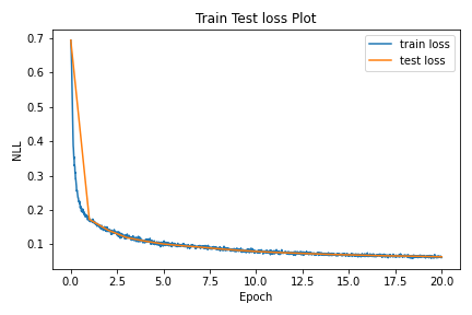
Figure 4: Train and Test loss curves
When the trained model is sampled to produce 100 synthetic images, we see that images produced are very similar to the inputs confirming that model has learnt well to create geometric shapes.
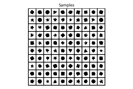
Figure 5: Images generated from trained model
This completes the deep dive into MADE model. The code can be found in accompanying github repository.