

In this post we will cover the concept of model interpretability. We will talk about its increasing importance as newer AI driven systems are getting adopted for critical and high impact scenarios. After the introduction, we will look into some popular approaches toward making complex model explainable.
This post is divided into following sections:
- Introduction
- Interpretable models
- Blackbox models
- Next steps and Conclusion
1. Introduction
With the growth of AI and Deep learning two things are happening today. On one side the ML models are becoming more and more complex e.g. BERT and GPT3 for language modelling. And then the 2nd thing is that the models are being deployed in many critical areas e.g. identification of suspects in crime, almost all financial decisions, e.g. granting a loan or a credit limit, insurance etc.
Till yesterday, it was ok for a model to work fine on test data before deployment and it was ok if the model could not be explained in terms of the predictions it was making, e.g. why a person was granted a loan and why was other person not granted? Or Why was the person identified as a threat based on facial analysis. Till yesterday, it was ok for the model to learn the biases present in the data, e.g. assigning lower probability of loan default to a white person.
However, as AI systems are being put more and more into daily use with far reaching impacts, there is an increasing demand from regulators and the society for the AI models to be:
a. Explainable
b. Free of biases
c. Trustworthy
And with the complexity of models going up, it is increasingly getting difficult to explain the predictions in terms that a human can understand. This has necessitated the development of the field of Interpretable ML. Once a model can be interpreted, its predictions can be explained. It can also be checked and hence corrected for the biases.
Regulators across all domains and countries have started demanding that decisions taken based on AI model predictions must be explainable with EU’s GDPR being one of the best examples. Under GDPR, people have a right to know how and why model predicted a specific outcome – this is known as "right to explanation".
Having established the important of interpretability of model, we will now look at two broad classes of models. First the models which are by design explainable and 2nd the blackbox model approach to interpret large complex non linear models.
2.0 Interpretable Models
We will briefly talk about three models which are interpretable. These are Linear Regression, Logistic Regression and Decision Trees.
Let us first look at Linear regression (LR). In LR, we estimate the value of dependent variable [latex] y [/latex] based on feature inputs as given below:
[latex]
\begin{align*}
y=\beta_{0}+\beta_{1}x_{1}+\ldots+\beta_{p}x_{p}+\epsilon
\end{align*}
[/latex]
The betas ([latex] \beta{j} [/latex]) represents the weight accorded to each feature vector. It also tells the amount by this [latex] y [/latex] will change for a unit change in the feature vector, e.g. [latex] \beta{j} [/latex] is the amount by which [latex] y [/latex] will change when [latex] x_j [/latex] is changed by one unit.
Similar to above Logistic Regression also makes it easy to understand the impact on outcome for each unit of change in feature values. Logistic Regression predicts the probability of a sample belonging to a class vs predicting the absolute value. Like Linear regression we first calculate a value [latex] y [/latex] as given below:
[latex]
\begin{align*}
\hat{y}=\beta_{0}+\beta_{1}x_{1}+\ldots+\beta_{p}x_{p}
\end{align*}
[/latex]
We then take sigmoid of the [latex] y [/latex] to constrain the value between 0 and 1. The sigmoid of [latex] y [/latex] predicts the probability that sample [latex] x [/latex] belongs to category 1 vs category 0.
[latex]
\begin{align*}
P(y=1)=\frac{1}{1+exp(-(\beta_{0}+\beta_{1}x_{1}+\ldots+\beta_{p}x_{p}))}
\end{align*}
[/latex]
With simple math manipulation we can show that:
[latex]
\begin{align*}
\frac{P(y=1)}{1-P(y=1)}=odds=exp\left(\beta_{0}+\beta_{1}x_{1}+\ldots+\beta_{p}x_{p}\right)
\end{align*}
[/latex]
The ratio is also called the odds ratio. If we change the value of a factor say [latex] x_j [/latex] by one unit, the odds ratio will change by a factor of [latex] exp\left(\beta_j\right) [/latex]. It is very similar to Linear regression except for the introduction of non linearity of exponential function.
Finally, we look at decision trees which are by its very nature very interpretable. Let us look at an example of a decision tree which has been built on Iris dataset, a dataset containing 150 samples each of 4 numeric values(sepal length, sepal width, petal length, petal width) across 3 types of iris-plants: Iris-Setosa, Iris-Versicolour, Iris-Virginica.
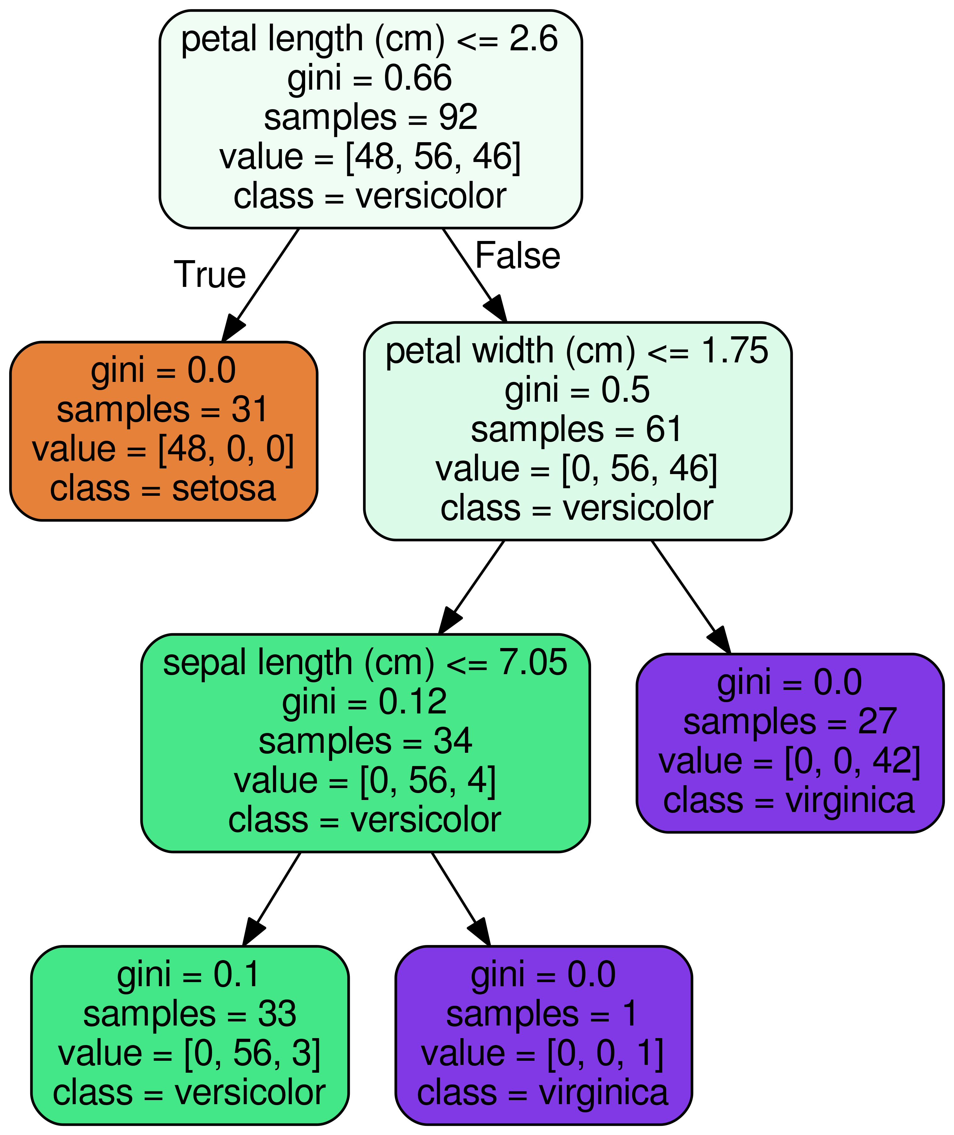
Figure 1: Decision Tree Classifier on IRIS dataset
The figure shows us that whenever a specific data point is predicted as belonging to one of the three classes, what attribute values contributed to that decision. As we walk down the tree from root node to leaf node, we can see the path we take to classify a specific datapoint. Let us look at the orange node in the above figure. If petal length is less than 2.6 cm, the tree will predict the sample to belong to Iris-setosa class.
3.0 Blackbox Models
Last section, we looked at some of the inherently interpretable models. However, with the advent of more powerful algorithms and abundance of data, the models are getting more and more complex. Even linear models or decision trees have too many features for human’s to comprehend it in an easy/intuitive way. The problem is further compounded with Deep learning where it is getting increasingly harder to explain the predictions made by the models in an easy to understand way. For Convolutional Neural Networks (CNN) in computer vision, we try to explain the network with the help of filters that the network learns at each layer. While that helps us talk at a generic level on what the network is learning, it still does not explain why a specific input resulted in a specific prediction. What factor contributed to what an extent in making that prediction. An example of such an explanation is show in figure 2.
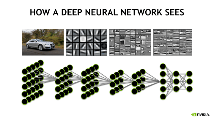
Figure 2: How does a Deep Neural network see
In this section we will look at some popular approaches that have found traction in helping explain the models. However, please note that these are early days of model interpretability. Even Azure has a library covering some of these approaches but the library is still in preview mode. You can read more about it here
3.1 Permutation Feature Importance
As explained in the book on Interpretable machine learning and the original paper by Breiman (2001) for Random Forests and as subsequently expanded into model-agnostic version by Fisher, Rudin, and Dominici (2018), the idea is very simple.
Consider that we have trained a model [latex] f [/latex] using n samples of p-dimensional data i.e. feature matrix [latex] \boldsymbol{X} [/latex] of dimensions (n x p), one row for each sample and each sample has p features, along with the labels/output [latex] y [/latex] of length n. Suppose we are interested in a metric like Mean Square Loss (MSE).
We first train the model [latex] f [/latex] on the training data [latex] \boldsymbol{X} [/latex] and [latex] y [/latex]. We calculate the MSE loss: [latex] loss\_{org} [/latex]
Now suppose, we want to assess the importance of the [latex] j^{th} [/latex] feature i.e. [latex] j^{th} [/latex] column of the input feature matrix [latex] \boldsymbol{X} [/latex]. We permute the values of the column [latex] x*j [/latex] so that we break the relationship between that feature [latex] x_j [/latex] and output labels [latex] y [/latex]. We then use the earlier pre-trained model to recalculate the MSE loss [latex] loss*{j} [/latex]. Please note that we do not train the model again.
The ratio of [latex] \frac{loss*{j}}{loss*{org}} [/latex] will tell us the importance of feature dimension [latex] x_j [/latex] in model prediction. Higher the value of the fraction, higher is the impact of permutating the feature dimension [latex] j [/latex]. Such a permutation results in higher loss and hence lesser quality prediction metric. That is just another way of saying that importance of feature [latex] x_j [/latex] is high in overall prediction.
Let us say the ratio stays at/around 1.0. What this means is that permutating feature [latex] x_j [/latex] did not impact the prediction and hence it can be concluded that feature [latex] j [/latex] did not contribute anything significant in the model’s prediction.
3.2 Global Surrogate
The approach under global Surrogate model is very simple. Suppose we have trained a blackbox model [latex] \boldsymbol{f} [/latex] which we want to interpret. We design a surrogate model [latex] \boldsymbol{g} [/latex]. This surrogate model [latex] \boldsymbol{g} [/latex] must belong to a class of interpretable models such as linear regression, logistic regression or decision tree which is trained using the output/predictions made by the actual trained model [latex] \boldsymbol{f} [/latex]. To check the quality of surrogate mode [latex] \boldsymbol{g} [/latex], we can calculate the measure [latex] R^2 [/latex] between the surrogate model [latex] \boldsymbol{g} [/latex] and the original blackbox model [latex] \boldsymbol{f} [/latex]. if [latex] R^2 [/latex] is close to 1.0, then surrogate model explains the original model well. We can use the interpretable surrogate model [latex] \boldsymbol{g} [/latex] to explain the predictions being made by the blackbox model [latex] \boldsymbol{f} [/latex].
3.3 Local Surrogate (LIME)
Next in the line is Local Surrogate model. It is very similar to surrogate model we talked about in previous section. The key difference is that under LIME, the surrogate model is trained to explain individual predictions. The learned surrogate model is a linear/interpretable model which is good approximation to the original blackbox model locally around the data point we want to explain but does not have a good global approximation. In other words, it has a good local fidelity. The approach was introduced in a paper titled “Why Should I Trust You?” Explaining the Predictions of Any Classifier which can be found here.
A toy example of LIME approach is shown in figure 2. The black-box model’s decision regions for 2-class classifier is shown as pink/blue region for the two classes. This boundary/region is not known to LIME. The bold red colored "+" is the individual point we want to explain. The dash line is the LIME learned model/explanation which is a good local approximation to the bold red "+" but is not a good global approximation.
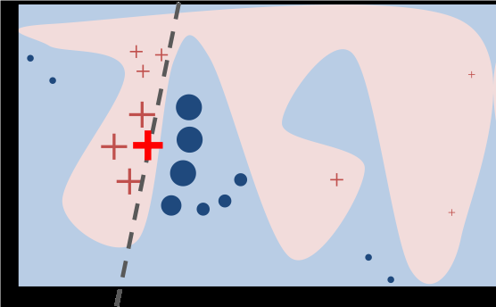
Figure 3: Toy example of LIME
Figure 4 shows the Explanation for an image classification prediction made by Google’s Inception neural network. The top 3 classes predicted are “Electric Guitar” (p = 0.32), “Acoustic guitar” (p = 0.24) and “Labrador” (p = 0.21)
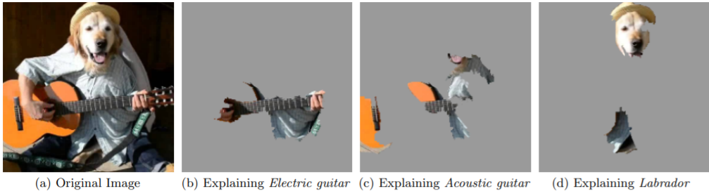
Figure 4: Explaining an image classification prediction made by Google’s Inception neural network. The top 3 classes predicted are “Electric Guitar” (p = 0.32), “Acoustic guitar” (p = 0.24) and “Labrador” (p = 0.21).
The paper also highlights the fact that interpretable model can help in identifying the hidden issues in the training data which can come to light when we try to explain a model. Let us consider a scenario. Assume that you are trying to use some patient data to make a prediction about the possibility of patient developing cancer in next five years. Amongst other dimensions, the input also has patient_id and part of the id is an identifier if the patient ever visited a caner specialist in the hospital in past. The algorithm may land up learning to use patient_id in making predictions about cancer probability. But this is not a real attribute and it will probably not be not present in actual live data once the system is deployed.
Using an interpretable approach, we will discover that prediction of outcome has a high weight on patient_id. On further exploration, either we will discover the source of data drift or we will decide to drop patient_id from training data to train the model. Whatever be the approach, an interpretable model not only helps us build trust with the end users, but also helps us catch errors such as data drifts and/or data leakages to be caught earlier.
LIME can also be used to explain deep learning models based on word embeddings and / or CNN based image classifiers. In case of images, the algorithm splits the images into small sub sections called super-pixels. The super-pixels (i.e. regions) are greyed out in different permutations to assess how that impacts the over-all prediction.
3.4 SHapley Additive exPlanations (SHAP)
Finally, we will talk about a game theory based approach called Shapley Additive Explanations (SHAP). This is one of the approaches available in multiple flavors inside Azure Machine Learning. You can read more about it here. The approach is based on a community driven development sponsored by Microsoft. The github repository for the same can be found here.
SHAP (SHapley Additive exPlanations) is a game theoretic approach to explain the output of any machine learning model. It connects optimal credit allocation with local explanations using the classic Shapley values from game theory and their related extensions. FOr further details on how this approach works, you can checkout the original paper from NIPS 2017 (Neural Information Processing Systems) here.
Let us look at Boston housing price dataset. It contains the price of 506 Boston suburb houses. There 13 factors recorded for each house along with median value of the house. We build a model to predict the price based on these 13 feature values ranging from crime rate to distance to employment centers. You can read more about this dataset here.
We use SHAP to explain the trained model as shown in figure 5 which shows features contributing to push the model output for a specific input from the base value. Base value is the average model prediction across the whole training set. Features pushing the prediction higher are shown in red, those pushing the prediction lower are in blue.
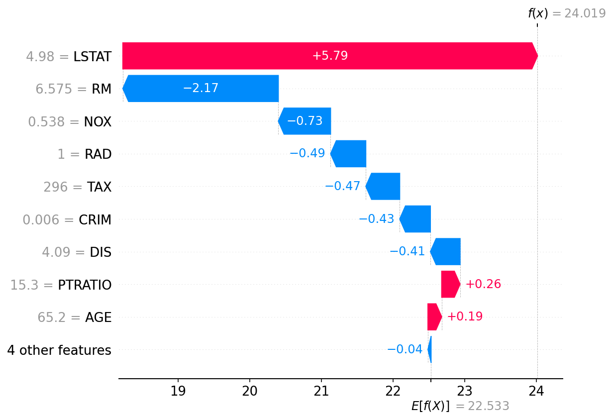
Figure 5: SHAP Explanation for Boston housing dataset.
4. Next steps and Conclusion
To conclude, model explainability is becoming important. In times to come, it will probably become part of many laws wherein the services using ML models would need to be able to explain to governments, regulators and users the decisions being made by the model.
To explore further the concepts we talked about in this post, pleas refer to following resources:
- Model interpretability in Azure
- Book on Interpretable machine learning
- Why Should I Trust You?” Explaining the Predictions of Any Classifier which can be found here. You can checkout the implementation of LIME at a github repository here
- SHAP (SHapley Additive exPlanations) paper here and a github repository supporting the same here.
I hope you enjoyed this post. I plan to expand on this post with detailed walkthroughs. Please stay tuned.