Hello , readers , I’m back again with my finance and trading series and sorry for not posting in the last week , got a little too caught up with the deadlines .Today we are going to use a python library that we use internally at Cloudcraftz Solutions Pvt. Ltd. for various experiments . Today we are going to see how to put that library to use for trading . This is a very simple strategy that we’ll be using to trade . So let’s start .
Note: If you’re wondering how to get this library , simply install using
pip install cloudcraftz.
import pandas as pd
import matplotlib.pyplot as plt
import numpy as np
import yfinance as yf

from cloudcraftz.technical_indicators import simple_moving_average, exponential_moving_average
from cloudcraftz.optimizers import sma_optimizer, ema_optimizer
from cloudcraftz.plots import cc_plot
from cloudcraftz.utils import split_func, get_signal_strategy, analyze_strategy, get_benchmark_result
Loading the price data from yahoo finance
df = yf.download("TCS", "2007-01-01", "2022-03-31")
[*********************100%***********************] 1 of 1 completed
df.tail()

So we have gathered the data , now we want to invest in TCS . So to replicate a real life trading scenario we will at the very beginning hold out a portion of the data which will serve as the unseen data for us .
Today we will be mainly using two technical indicators namely SMA and EMA . (Simple and Exponential Moving Averages (MA — abbreviated)).
# We'll be taking the close price as our price , assuming that we buy or sell at close .

train_X, test_X = split_func(df['Close'], test_size=0.2)
train_X.head()
Date
2013-11-01    36.200001
2013-11-04    35.349998
2013-11-05    35.349998
2013-11-06    35.900002
2013-11-07    35.310001
Name: Close, dtype: float64
There are many rules that are used by traders such as 5-day SMA signal or 8-day EMA signal, but rather relying on those we will let our library function decide which is best for us , here we will use the crossover strategy , Crossovers are one of the main moving average strategies. The first type is a price crossover, which is when the price crosses above or below a moving average to signal a potential change in trend. Say for example a 5-day moving average crosses over a 20-day moving average, then it signifies a strong trend of the presence of a bull market, because the 5 day moving average is giving us a very recent smoothened price of the stock as compared to a 20 day MA .
# Let's get the optimum time periods for our stock , we'll be using both SMA and EMA signals to trade .
t1_sma, t2_sma, sma = sma_optimizer(train_X)
t1_ema, t2_ema, ema = ema_optimizer(train_X)
So we have got the optimal signal along with the optimal periods, we don’t have to do anything we just pass the prices and it does all the optimisations internally and spits out the results. Now comes the fun part , to simulate a real trading scenario we will take one row of the held out set at a time which will serve as each passing day .
old_data = list(train_X.values)
def signals(close):
    old_data.append(close)
    sma_short = simple_moving_average(old_data, {'periods': t1_sma})
    sma_long = simple_moving_average(old_data, {'periods': t2_sma})
    sig_today_sma = get_signal_strategy(sma_short, sma_long)

    ema_short = exponential_moving_average(old_data, {'periods': t1_ema})
    ema_long = exponential_moving_average(old_data, {'periods': t2_ema})
    sig_today_ema = get_signal_strategy(ema_short, ema_long)

    one, two = sig_today_sma[-1], sig_today_ema[-1]

    sig = 0.6 * two + 0.4 * one

    if sig >= 0.5:
        return 1
    elif sig <= -0.5:
        return -1
    else:
        return 0
We got our function ready which gives us the SMA and EMA signals for that particular day , given the closing price or the buying price of that day . Now we know , that EMA or Exponential MA is very sensitive to price changes, so we give a 60% weight to that signal and 40% to our SMA signal . We have used 0.5 as our threshold for deciding whether to buy or not to buy or to hold (1, -1 or 0)
What we are doing below is passing through each day (used a for loop for that) we get the price each day and pass it through our function signals to recieve the action that we must take on that particular day .
# We keep a list to keep track of our action , that is buy sell or hold
actions = []

for prices in test_X.values:
    action = signals(prices)
    actions.append(action)
Evaluation of our strategy
For that we will be using the analyze_strategy function in the cloudcraftz’s utils module .
Note: Below before passing our data to
analyze_strategyfunction , we did a reset to make the date index as column and also renamed theClosecolumn topricesor else it’ll give an error . (Read the doc-string before using the library functions).
# pass the list of actions taken and the prices of each day with their dates.
prices = test_X.reset_index()
prices.rename(columns={"Close": "prices"}, inplace=True)

analyze_strategy(actions, prices, plot=True)


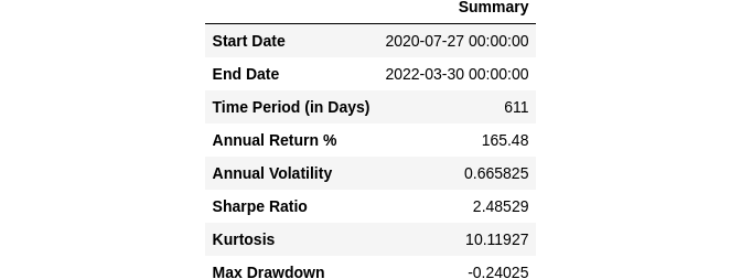
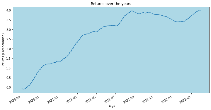
WoW ! we got a return of 165% , so had we used this strategy to trade for the given period we would have made 2.65 times more of what we invested . That actually makes sense as well since TCS is a IT company , for the period we are testing our strategy on, the prices actually had an upward trend for all IT based companies . But the question is did we actually did better as compared to the index ? I mean we need to have something to compare our strategy with right ? Let’s compare it with NIFTY50 to see how it performed .
get_benchmark_result("^NSEI", "2020-07-27", "2022-03-31")
[*********************100%***********************] 1 of 1 completed

Amazing so we are beating the market by 8 times, the NIFTY50 index had an Annual return of 23.59% whereas we with our strategy have 165% , which is extremely good .
So the result that we got is too good , you may try this out on other stocks as well , though I’m kind of not sure if it’ll produce such good results , since it is a very simple strategy , try it out on various stocks from different industries to see how well it performs before you start investing in real time .
Thank you geeks , I hope you enjoyed this article , do let me know in the comments if you want to see more such posts , till then see ya geeks !!

