Hello , readers, today I’m back with another interesting post . As you might know this is the time IPL (Indian Premiere League)is going on and so I decided to built a model so that I can predict what is going to happen in the very next ball and earn some money by gambling , “haha sorry I was joking !”(Never Gamble that’s bad ). Jokes apart today we are going to see how we can built a ML model that predicts what is going happen in the next ball .
So let’s begin and see what story our data has to tell us today ! Be patient because this post is going to be a long one .
Import Statements
import warnings
import xgboost as xgb
warnings.filterwarnings('ignore')
import pandas as pd
import numpy as np
import matplotlib.pyplot as plt
import seaborn as sns
from sklearn.preprocessing import LabelEncoder
from sklearn.model_selection import train_test_split
from sklearn.metrics import accuracy_score, plot_confusion_matrix, confusion_matrix
Data Loading , Cleaning and Manipulations
cric = pd.read_csv('all_matches.csv')
The format of the data
The first row of each CSV file contains the headers for the file, with each subsequent row providing details on a single delivery. The headers in the file are:
- match_id
- season
- start_date
- venue
- innings
- ball
- batting_team
- bowling_team
- striker
- non_striker
- bowler
- runs_off_bat
- extras
- wides
- noballs
- byes
- legbyes
- penalty
- wicket_type
- player_dismissed
- other_wicket_type
- other_player_dismissed
Most of the fields above should, hopefully, be self-explanatory, but some may benefit from clarification…
“innings” contains the number of the innings within the match. If a match is one that would normally have 2 innings, such as a T20 or ODI, then any innings of more than 2 can be regarded as a super over.
“ball” is a combination of the over and delivery. For example, “0.3” represents the 3rd ball of the 1st over.
“wides”, “noballs”, “byes”, “legbyes”, and “penalty” contain the total of each particular type of extras, or are blank if not relevant to the delivery.
If a wicket occurred on a delivery then “wicket_type” will contain the method of dismissal, while “player_dismissed” will indicate who was dismissed. There is also the, admittedly remote, possibility that a second dismissal can be recorded on the delivery (such as when a player retires on the same delivery as another dismissal occurs). In this case “other_wicket_type” will record the reason, while “other_player_dismissed” will show who was dismissed.
cric.head()

cric.tail()

Let’s see the shape to get some idea regarding the size of our dataset .
cric.shape
(194354, 22)
Let’s have a look at the dtypes of the dataset columns as well .
cric.info()
<class 'pandas.core.frame.DataFrame'>
RangeIndex: 194354 entries, 0 to 194353
Data columns (total 22 columns):
 #   Column                  Non-Null Count   Dtype
---  ------                  --------------   -----
 0   match_id                194354 non-null  int64
 1   season                  194354 non-null  object
 2   start_date              194354 non-null  object
 3   venue                   194354 non-null  object
 4   innings                 194354 non-null  int64
 5   ball                    194354 non-null  float64
 6   batting_team            194354 non-null  object
 7   bowling_team            194354 non-null  object
 8   striker                 194354 non-null  object
 9   non_striker             194354 non-null  object
 10  bowler                  194354 non-null  object
 11  runs_off_bat            194354 non-null  int64
 12  extras                  194354 non-null  int64
 13  wides                   5884 non-null    float64
 14  noballs                 774 non-null     float64
 15  byes                    511 non-null     float64
 16  legbyes                 3118 non-null    float64
 17  penalty                 2 non-null       float64
 18  wicket_type             9560 non-null    object
 19  player_dismissed        9560 non-null    object
 20  other_wicket_type       0 non-null       float64
 21  other_player_dismissed  0 non-null       float64
dtypes: float64(8), int64(4), object(10)
memory usage: 32.6+ MB
### Check for Missing data

cric.isnull().sum()
match_id                       0
season                         0
start_date                     0
venue                          0
innings                        0
ball                           0
batting_team                   0
bowling_team                   0
striker                        0
non_striker                    0
bowler                         0
runs_off_bat                   0
extras                         0
wides                     188470
noballs                   193580
byes                      193843
legbyes                   191236
penalty                   194352
wicket_type               184794
player_dismissed          184794
other_wicket_type         194354
other_player_dismissed    194354
dtype: int64
Most of the missing values are from the columns such as noballs , byes etc . So they represent that no such event took place in that particular delivery , so that can be easily filled by replacing NaN with 0.
cric.fillna(0, inplace=True)
cric.head()

cric.info()
<class 'pandas.core.frame.DataFrame'>
RangeIndex: 194354 entries, 0 to 194353
Data columns (total 22 columns):
 #   Column                  Non-Null Count   Dtype
---  ------                  --------------   -----
 0   match_id                194354 non-null  int64
 1   season                  194354 non-null  object
 2   start_date              194354 non-null  object
 3   venue                   194354 non-null  object
 4   innings                 194354 non-null  int64
 5   ball                    194354 non-null  float64
 6   batting_team            194354 non-null  object
 7   bowling_team            194354 non-null  object
 8   striker                 194354 non-null  object
 9   non_striker             194354 non-null  object
 10  bowler                  194354 non-null  object
 11  runs_off_bat            194354 non-null  int64
 12  extras                  194354 non-null  int64
 13  wides                   194354 non-null  float64
 14  noballs                 194354 non-null  float64
 15  byes                    194354 non-null  float64
 16  legbyes                 194354 non-null  float64
 17  penalty                 194354 non-null  float64
 18  wicket_type             194354 non-null  object
 19  player_dismissed        194354 non-null  object
 20  other_wicket_type       194354 non-null  float64
 21  other_player_dismissed  194354 non-null  float64
dtypes: float64(8), int64(4), object(10)
memory usage: 32.6+ MB
Exploratory Data Analysis and Feature Engineering
There are few things that are not needed atleast as far as analysis and predictions are concerned. Such as match_id, start_date , since they are mostly unique . Another reason for dropping the start_date is because we don’t the date of the match to have an influence on the predictions ,since a date occurs only once .
cric.drop(['match_id', 'start_date'], axis=1, inplace=True)
The describe method tell us a lot about the data .
cric.describe()

From the above table we can see that two other columns other_wicket_type and other_player_dismissed does not have any variation so they can dropped without any hesitation .
cric.drop(["other_wicket_type", "other_player_dismissed"], axis=1, inplace=True)
Seems like the feature player_dimissed is telling us who was dismissed in that particular ball . But if we want to know how much is my batsmen going to score in the next ball this feature is not particularly important , because telling our model that someone got dismissed in this ball and then asking “so what would be the run ?” It’s absurd , it’s like we already know the future who is going to get dismissed .
cric["player_dismissed"].unique()
array([0, 'SC Ganguly', 'RT Ponting', 'DJ Hussey', 'R Dravid', 'V Kohli',
       'JH Kallis', 'W Jaffer', 'MV Boucher', 'B Akhil', 'CL White',
       'AA Noffke', 'Z Khan', 'SB Joshi', 'PA Patel', 'ML Hayden',
       'MS Dhoni', 'SK Raina', 'JDP Oram', 'K Goel', 'JR Hopes',
       'Yuvraj Singh', 'KC Sangakkara', 'T Kohli', 'YK Pathan',
       'SR Watson', 'DS Lehmann', 'M Kaif', 'M Rawat', 'RA Jadeja',
       'SK Warne', 'V Sehwag', 'Y Venugopal Rao', 'VVS Laxman',
       'AC Gilchrist', 'RG Sharma', 'SB Styris', 'AS Yadav', 'A Symonds',
       'WPUJC Vaas', 'SB Bangar', 'PP Ojha', 'BB McCullum', 'WP Saha',
       'Mohammad Hafeez', 'L Ronchi', 'DJ Thornely', 'ST Jayasuriya',
       'PR Shah', 'RV Uthappa', 'AM Nayar', 'SM Pollock', 'S Chanderpaul',
       'LRPL Taylor', 'DPMD Jayawardene', 'IK Pathan', 'B Lee', 'S Sohal',
       'Kamran Akmal', 'Shahid Afridi', 'G Gambhir', 'MEK Hussey',
       'DJ Bravo', 'MA Khote', 'Harbhajan Singh', 'GC Smith',
       'D Salunkhe', 'RR Sarwan', 'PP Chawla', 'S Sreesanth', 'VRV Singh',
       'SS Tiwary', 'AB Agarkar', 'M Kartik', 'LR Shukla', 'P Kumar',
       'AM Rahane', 'S Dhawan', 'Shoaib Malik', 'KD Karthik', 'R Bhatia',
       'MK Tiwary', 'MF Maharoof', 'SM Katich', 'TM Srivastava',
       'B Chipli', 'DW Steyn', 'DB Das', 'MK Pandey', 'SA Asnodkar',
       'Salman Butt', 'BJ Hodge', 'Umar Gul', 'AB Dinda', 'HH Gibbs',
       'DNT Zoysa', 'D Kalyankrishna', 'SP Fleming', 'S Vidyut',
       'JA Morkel', 'SE Marsh', 'Misbah-ul-Haq', 'S Badrinath',
       'Joginder Sharma', 'M Muralitharan', 'M Ntini', 'YV Takawale',
       'AB de Villiers', 'PJ Sangwan', 'Mohammad Asif', 'GD McGrath',
       'DT Patil', 'A Kumble', 'S Anirudha', 'Sohail Tanvir',
       'SK Trivedi', 'CK Kapugedera', 'A Chopra', 'T Taibu',
       'J Arunkumar', 'DB Ravi Teja', 'RP Singh', 'A Mishra',
       'AD Mascarenhas', 'R Vinay Kumar', 'TM Dilshan', 'VY Mahesh',
       'SR Tendulkar', 'I Sharma', 'Shoaib Akhtar', 'LPC Silva', 'H Das',
       'SP Goswami', 'DR Smith', 'SD Chitnis', 'A Nehra', 'VS Yeligati',
       'MS Gony', 'L Balaji', 'LA Pomersbach', 'A Nel', 'A Mukund',
       'Younis Khan', 'Niraj Patel', 'WA Mota', 'JD Ryder',
       'KP Pietersen', 'T Henderson', 'MM Patel', 'Kamran Khan',
       'JP Duminy', 'A Flintoff', 'RS Bopara', 'CH Gayle', 'MC Henriques',
       'R Bishnoi', 'KV Sharma', 'PC Valthaty', 'RJ Quiney',
       'Yashpal Singh', 'Pankaj Singh', 'FH Edwards', 'AS Raut',
       'AN Ghosh', 'BAW Mendis', 'DL Vettori', 'RE van der Merwe',
       'RR Powar', 'AA Bilakhia', 'TL Suman', 'Shoaib Ahmed', 'GR Napier',
       'MN van Wyk', 'M Vijay', 'SB Jakati', 'DA Warner', 'M Manhas',
       'NV Ojha', 'LA Carseldine', 'RJ Harris', 'D du Preez', 'RR Raje',
       'DS Kulkarni', 'M Morkel', 'AD Mathews', 'C Nanda', 'SL Malinga',
       'S Tyagi', 'J Botha', 'A Singh', 'GJ Bailey', 'AB McDonald',
       'Y Nagar', 'SS Shaikh', 'R Ashwin', 'T Thushara',
       'Mohammad Ashraful', 'CA Pujara', 'Anirudh Singh', 'MS Bisla',
       'AP Tare', 'AT Rayudu', 'R Sathish', 'AA Jhunjhunwala', 'P Dogra',
       'A Uniyal', 'JM Kemp', 'EJG Morgan', 'OA Shah', 'RS Gavaskar',
       'SE Bond', 'KA Pollard', 'DP Nannes', 'MJ Lumb', 'DR Martyn',
       'S Narwal', 'AB Barath', 'FY Fazal', 'MD Mishra', 'S Ladda',
       'J Theron', 'SJ Srivastava', 'R Sharma', 'Mandeep Singh',
       'AC Voges', 'Jaskaran Singh', 'KAJ Roach', 'PD Collingwood',
       'CK Langeveldt', 'VS Malik', 'KM Jadhav', 'SW Tait', 'A Mithun',
       'AP Dole', 'Harmeet Singh', 'R McLaren', 'S Sriram', 'KP Appanna',
       'C Madan', 'AG Paunikar', 'MR Marsh', 'AJ Finch', 'STR Binny',
       'B Sumanth', 'IR Jaggi', 'DT Christian', 'RV Gomez', 'MA Agarwal',
       'Sunny Singh', 'UBT Chand', 'UT Yadav', 'DJ Jacobs', 'AL Menaria',
       'AUK Pathan', 'WD Parnell', 'JJ van der Wath', 'R Ninan',
       'MS Wade', 'TD Paine', 'SB Wagh', 'JEC Franklin',
       'Shakib Al Hasan', 'BJ Haddin', 'S Randiv', 'NLTC Perera',
       'JE Taylor', 'NL McCullum', 'RN ten Doeschate', 'TR Birt',
       'M Klinger', 'Harpreet Singh', 'Bipul Sharma', 'AC Blizzard',
       'CA Ingram', 'S Nadeem', 'DH Yagnik', 'KB Arun Karthik',
       'AA Chavan', 'ND Doshi', 'CJ Ferguson', 'Y Gnaneswara Rao',
       'S Rana', 'BA Bhatt', 'F du Plessis', 'DE Bollinger', 'RE Levi',
       'MN Samuels', 'B Kumar', 'SPD Smith', 'SA Yadav', 'DJ Harris',
       'Ankit Sharma', 'HV Patel', 'GJ Maxwell', 'JP Faulkner',
       'SP Narine', 'KK Cooper', 'GB Hogg', 'RR Bhatkal', 'CJ McKay',
       'N Saini', 'DA Miller', 'P Negi', 'Azhar Mahmood', 'AC Thomas',
       'RJ Peterson', 'A Ashish Reddy', 'V Pratap Singh', 'MJ Clarke',
       'Gurkeerat Singh', 'VR Aaron', 'PA Reddy', 'AP Majumdar',
       'AD Russell', 'CA Lynn', 'Sunny Gupta', 'MC Juneja', 'KK Nair',
       'GH Vihari', 'MDKJ Perera', 'B Laughlin', 'Mohammed Shami',
       'BMAJ Mendis', 'M Vohra', 'R Rampaul', 'P Awana',
       'SMSM Senanayake', 'BJ Rohrer', 'KL Rahul', 'J Syed Mohammad',
       'Q de Kock', 'BB Samantray', 'R Dhawan', 'MG Johnson', 'LJ Wright',
       'AG Murtaza', 'IC Pandey', 'X Thalaivan Sargunam', 'DJG Sammy',
       'SV Samson', 'KW Richardson', 'CH Morris', 'MM Sharma',
       'CM Gautam', 'UA Birla', 'Parvez Rasool', 'Sachin Baby',
       'NM Coulter-Nile', 'CJ Anderson', 'NJ Maddinson', 'AR Patel',
       'JDS Neesham', 'TG Southee', 'PV Tambe', 'MA Starc', 'BR Dunk',
       'RR Rossouw', 'Shivam Sharma', 'LMP Simmons', 'VH Zol',
       'BCJ Cutting', 'Imran Tahir', 'R Shukla', 'BE Hendricks',
       'M de Lange', 'S Gopal', 'R Tewatia', 'JO Holder', 'JD Unadkat',
       'Iqbal Abdulla', 'SS Iyer', 'DJ Hooda', 'SN Khan', 'D Wiese',
       'HH Pandya', 'MJ McClenaghan', 'SA Abbott', 'AN Ahmed',
       'KS Williamson', 'Anureet Singh', 'DJ Muthuswami', 'PJ Cummins',
       'Karanveer Singh', 'Sandeep Sharma', 'J Suchith', 'JC Buttler',
       'CR Brathwaite', 'MP Stoinis', 'Ishan Kishan', 'C Munro',
       'AD Nath', 'MJ Guptill', 'P Sahu', 'TM Head', 'M Ashwin',
       'KH Pandya', 'NS Naik', 'RR Pant', 'SW Billings', 'KC Cariappa',
       'PSP Handscomb', 'Swapnil Singh', 'J Yadav', 'UT Khawaja',
       'HM Amla', 'JJ Bumrah', 'A Zampa', 'N Rana', 'S Kaushik',
       'F Behardien', 'KJ Abbott', 'ER Dwivedi', 'CJ Jordan', 'S Aravind',
       'TS Mills', 'YS Chahal', 'BA Stokes', 'JJ Roy', 'Vishnu Vinod',
       'CR Woakes', 'RA Tripathi', 'DL Chahar', 'V Shankar',
       'Rashid Khan', 'SN Thakur', 'C de Grandhomme', 'S Badree',
       'AF Milne', 'Mohammad Nabi', 'K Rabada', 'AJ Tye', 'Kuldeep Yadav',
       'SP Jackson', 'Ankit Soni', 'A Choudhary', 'AS Rajpoot',
       'Washington Sundar', 'MM Ali', 'SO Hetmyer', 'S Dube', 'NA Saini',
       'JM Bairstow', 'PP Shaw', 'KMA Paul', 'N Pooran', 'JC Archer',
       'K Gowtham', 'M Markande', 'Shubman Gill', 'P Ray Barman',
       'SM Curran', 'GC Viljoen', 'S Lamichhane', 'RD Chahar', 'S Kaul',
       'Mohammed Siraj', 'M Prasidh Krishna', 'SD Lad', 'R Parag',
       'JL Denly', 'LS Livingstone', 'RK Bhui', 'Abhishek Sharma',
       'KK Ahmed', 'AJ Turner', 'E Lewis', 'MA Wood', 'RK Singh',
       'DJM Short', 'Mujeeb Ur Rahman', 'Shivam Mavi', 'TK Curran',
       'TA Boult', 'H Klaasen', 'LE Plunkett', 'Basil Thampi',
       'Mustafizur Rahman', 'BB Sran', 'AD Hales', 'MK Lomror',
       'DR Shorey', 'P Chopra', 'IS Sodhi', 'JPR Scantlebury-Searles',
       'SE Rutherford', 'MJ Santner', 'P Simran Singh', 'JL Pattinson',
       'D Padikkal', 'PK Garg', 'YBK Jaiswal', 'RD Gaikwad',
       'JR Philippe', 'Ravi Bishnoi', 'Abdul Samad', 'I Udana',
       'KL Nagarkoti', 'CV Varun', 'SS Cottrell', 'Arshdeep Singh',
       'N Jagadeesan', 'T Banton', 'AT Carey', 'TU Deshpande', 'A Nortje',
       'Kartik Tyagi', 'DR Sams', 'M Jansen', 'RM Patidar',
       'Shahbaz Ahmed', 'KA Jamieson'], dtype=object)
# So we drop the column "player_dismissed" as well .
cric.drop("player_dismissed", axis=1, inplace=True)
With the same logic as above it is not possible to tell before a bowl has been delivered, that whether it’s going to be a wide-ball or a no-ball or even the wicket_type or legbyes etc.
cric.columns
Index(['season', 'venue', 'innings', 'ball', 'batting_team', 'bowling_team',
       'striker', 'non_striker', 'bowler', 'runs_off_bat', 'extras', 'wides',
       'noballs', 'byes', 'legbyes', 'penalty', 'wicket_type'],
      dtype='object')
# So we drop those features as well
cric.drop(cric.columns[-7:], axis=1, inplace=True)
Now after a lot of analysis with our basic knowledge of the game “cricket” we have a dataframe that is free of many features that were not needed for the problem that we are trying to solve.
cric.head()

Advanced Data Analysis
Let’s see how the over number is affecting the scores of the bat .
# create a variable to store the over number
over_number = cric["ball"].astype("str")
overs = []

for i in over_number.values:
    overs.append(int(i.split('.')[0]))
# let's append the column overs to the original dataframe

df = pd.concat([cric, pd.Series(overs)], axis=1)
df.rename(columns={df.columns[-1]: "over_n"}, inplace=True)
LET US SEE THE RUNS OFF THE BAT (AVG RUN) BASED ON THE OVER BEING PLAYED
df.groupby("over_n").mean()[["runs_off_bat"]].plot(figsize=(15, 8), style="k--")
<AxesSubplot:xlabel='over_n'>
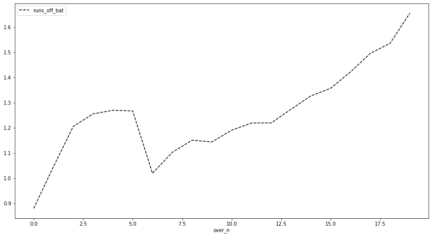
Some interesting observations:
- The runs scored are highest in the slog overs (towards the end).
- The runs take a peak from the 3rd over till almost the 6th over and then falls drastically most probably due to the reason that the powerplay restrictions are taken off after the 6th over.
- The runs again starts gaining momentum after the 7 or the 8th over .
Let’s see how the season is affecting the scores of the bat .
df["season"] = df["season"].astype('str')
temp = df.season.unique()
# But let's first do some manipulations , convertions are quite self-explanatory since some seasons are in 2009/10 etc format and some are in
# 2012 etc format that might make it difficult for analysis .

for i in range(len(df)):
    if df.iloc[i, 0] == temp[0]:
        df.iloc[i, 0] = "2007"
    elif df.iloc[i, 0] == temp[2]:
        df.iloc[i, 0] == "2010"
    elif df.iloc[i, 0] == temp[-2]:
        df.iloc[i, 0] == "2020"
df.head()

df.groupby("season").mean()['runs_off_bat'].plot(figsize=(15, 8), style="r--")
<AxesSubplot:xlabel='season'>
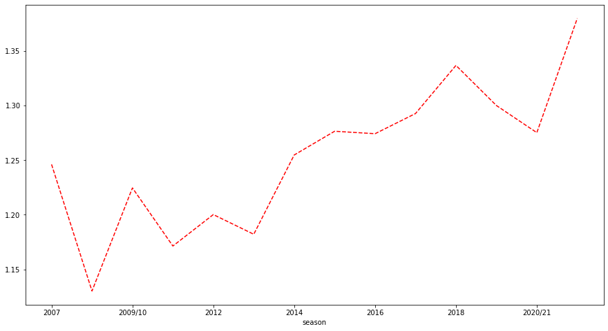
Doesn’t seem like there is a pattern , but still let’s do some more analysis before we reach any conclusions .
Let’s see if the runs scored in a over has any effect of the season .
df.groupby(["season", "over_n"]).mean()['runs_off_bat'].plot(figsize=(15, 8), style="g--")
<AxesSubplot:xlabel='season,over_n'>
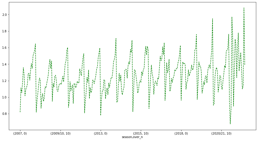
Observation:
- Irrespective of what the season is , the curve clearly shows it follows the same pattern .
So I guess we can drop the season parameter .
df.drop("season", axis=1, inplace=True)
df.tail()

Scoring depends on bats-person(men or women), bowlers , the venue where it is being played since the pitch plays an important role.
Let’s not keep any stoned unturned .
# Let's see the mean score by venues

dw = df.groupby("venue").mean()["runs_off_bat"].sort_values()
y_pos = dw.values
y_index = dw.index
plt.figure(figsize=(8, 16))
plt.barh(y_index, y_pos)
plt.ylabel('Venues')
plt.xlabel('Average Runs')
plt.title('Venue vs Avg Runs Scored Per ball')
Text(0.5, 1.0, 'Venue vs Avg Runs Scored Per ball')

Let’s now see the effect of innings vs average runs scored .
df.groupby(["innings"]).mean()['runs_off_bat'].plot(figsize=(12, 6), style="y--")
<AxesSubplot:xlabel='innings'>
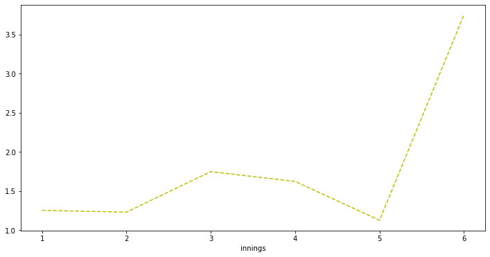
Very clearly super-over innings are just over-powered , pressure is more , lesser deliveries more runs have to be scored , quite an expected graph .
The last thing we would love to see if we are not missing out on anything else is that how the batting and bowling teams are influencing the runs per ball , because players leave and join other teams so the roaster keeps changing . This one is the most trickiest part, because on one hand the roasters keep udpdating and on the other hand bowling team’s fielding capabilities plays an important role in keeping the runs at check.
dh = df.groupby("bowling_team").mean()["runs_off_bat"].sort_values()
c_pos = dh.values
c_index = dh.index
plt.figure(figsize=(14, 5))
plt.barh(c_index, c_pos, color=['red', 'yellow', 'green', 'blue', 'orange'])
plt.ylabel('Bowling Teams')
plt.xlabel('Average Runs')
plt.title('Bowling Team vs Avg Runs Scored Per ball')
Text(0.5, 1.0, 'Bowling Team vs Avg Runs Scored Per ball')
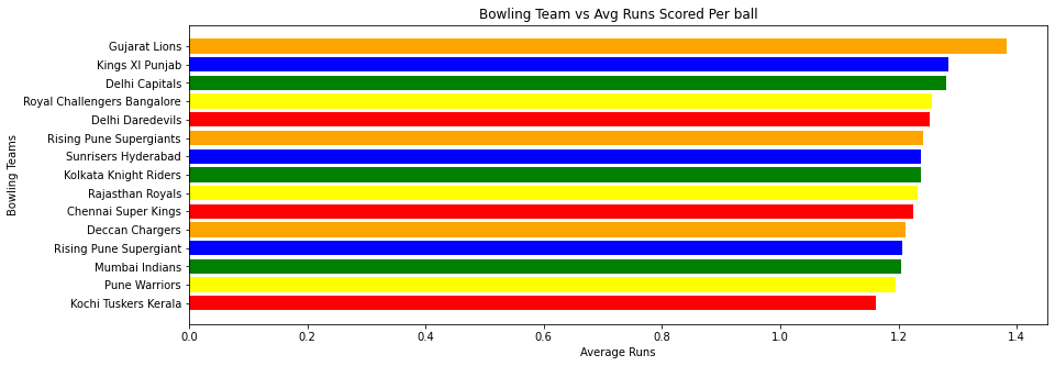
dh.describe()
count    15.000000
mean      1.240921
std       0.050756
min       1.162330
25%       1.209163
50%       1.237471
75%       1.254904
max       1.382793
Name: runs_off_bat, dtype: float64
Let’s see this together with season to understand the effet better .
cric.groupby(["season", "bowling_team"]).mean()["runs_off_bat"].loc[('2009')].plot(figsize=(14, 8))
cric.groupby(["season", "bowling_team"]).mean()["runs_off_bat"].loc[('2012')].plot(figsize=(14, 8))
cric.groupby(["season", "bowling_team"]).mean()["runs_off_bat"].loc[('2018')].plot(figsize=(14, 8))
plt.xticks(rotation=90)
(array([-1.,  0.,  1.,  2.,  3.,  4.,  5.,  6.,  7.,  8.]),
 [Text(-1.0, 0, 'Sunrisers Hyderabad'),
  Text(0.0, 0, 'Chennai Super Kings'),
  Text(1.0, 0, 'Delhi Daredevils'),
  Text(2.0, 0, 'Kings XI Punjab'),
  Text(3.0, 0, 'Kolkata Knight Riders'),
  Text(4.0, 0, 'Mumbai Indians'),
  Text(5.0, 0, 'Rajasthan Royals'),
  Text(6.0, 0, 'Royal Challengers Bangalore'),
  Text(7.0, 0, 'Sunrisers Hyderabad'),
  Text(8.0, 0, '')])
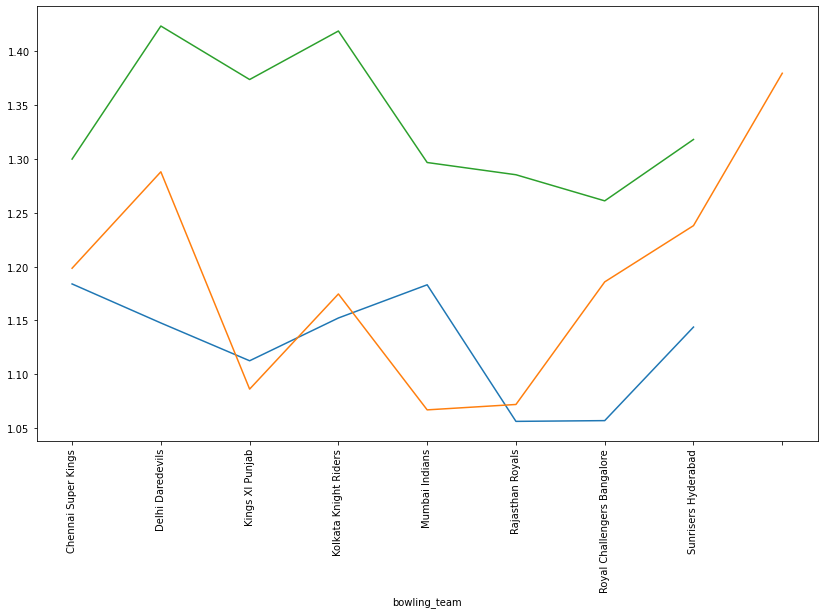
We can clearly see there some pattern every season, the bowling team seems to have a good effect on the outcome .
We’ll not check the outcome with that of the batting team because the bats-person is the person who is solely resposible for scoring, who is a part of the batting team
Data Splitting and Model Building
# Before we split the data we'll drop the "over_n" because it is highly correlated to the feature "ball", this may introduce multi-collinearity .

features = df.drop(["over_n", "runs_off_bat"], axis=1)
labels = df["runs_off_bat"]
# We've to encode the object type features to numerical types
enc_label = LabelEncoder()
We are converting these because the models are purely mathematical they don’t understand anything other than numbers .
features["batting_team"] = enc_label.fit_transform(features["batting_team"])
features["venue"] = enc_label.fit_transform(features["venue"])
features["bowling_team"] = enc_label.fit_transform(features["bowling_team"])
features["striker"] = enc_label.fit_transform(features["striker"])
features["non_striker"] = enc_label.fit_transform(features["non_striker"])
features["bowler"] = enc_label.fit_transform(features["bowler"])
features.shape
(194354, 8)
labels.shape
(194354,)
# let's now split our dataset
X_train, X_test, y_train, y_test = train_test_split(features, labels, test_size=0.2)
XGBClassifier Model for predicting the outcome
If we take a look we see that there only 7 unique outcomes , so we can frame this as a classification problem . A multi-class classification
labels.unique()
array([0, 4, 6, 1, 2, 5, 3])
xgb_model = xgb.XGBClassifier()
xgb_model.fit(X_train, y_train)
[21:20:45] WARNING: ../src/learner.cc:1115: Starting in XGBoost 1.3.0, the default evaluation metric used with the objective 'multi:softprob' was changed from 'merror' to 'mlogloss'. Explicitly set eval_metric if you'd like to restore the old behavior.


XGBClassifier(base_score=0.5, booster='gbtree', colsample_bylevel=1,
              colsample_bynode=1, colsample_bytree=1, enable_categorical=False,
              gamma=0, gpu_id=-1, importance_type=None,
              interaction_constraints='', learning_rate=0.300000012,
              max_delta_step=0, max_depth=6, min_child_weight=1, missing=nan,
              monotone_constraints='()', n_estimators=100, n_jobs=4,
              num_parallel_tree=1, objective='multi:softprob', predictor='auto',
              random_state=0, reg_alpha=0, reg_lambda=1, scale_pos_weight=None,
              subsample=1, tree_method='exact', validate_parameters=1,
              verbosity=None)
y_pred = xgb_model.predict(X_test)
print("The % Accuracy of the Model is: ", accuracy_score(y_test, y_pred) * 100)
The % Accuracy of the Model is: 46.04460909161071
The accuracy isn’t great, so let’s re-frame the problem , let’s say we are trying to predict if the next ball is going to be a ‘4’, ‘5’, ‘6’ or is it something between 0–3 . (That is a boundary or not a boundary)
- Let’s frame this as a binary classification problem
X = df.drop(["over_n", "runs_off_bat"], axis=1)
y = df["runs_off_bat"]
# Before we split the train and test sets lets change the labels

X["batting_team"] = enc_label.fit_transform(X["batting_team"])
X["venue"] = enc_label.fit_transform(X["venue"])
X["bowling_team"] = enc_label.fit_transform(X["bowling_team"])
X["striker"] = enc_label.fit_transform(X["striker"])
X["non_striker"] = enc_label.fit_transform(X["non_striker"])
X["bowler"] = enc_label.fit_transform(X["bowler"])
Y = np.zeros(y.shape)

for i in range(len(y)):
    if y[i] >= 4:
        Y[i] = 0
    else:
        Y[i] = 1
pd.Series(Y).value_counts()
1.0    163310
0.0     31044
dtype: int64
X_train, X_test, y_train, y_test = train_test_split(X, Y, test_size=0.2)
model = xgb.XGBClassifier()
model.fit(X_train, y_train)
[21:21:55] WARNING: ../src/learner.cc:1115: Starting in XGBoost 1.3.0, the default evaluation metric used with the objective 'binary:logistic' was changed from 'error' to 'logloss'. Explicitly set eval_metric if you'd like to restore the old behavior.


XGBClassifier(base_score=0.5, booster='gbtree', colsample_bylevel=1,
              colsample_bynode=1, colsample_bytree=1, enable_categorical=False,
              gamma=0, gpu_id=-1, importance_type=None,
              interaction_constraints='', learning_rate=0.300000012,
              max_delta_step=0, max_depth=6, min_child_weight=1, missing=nan,
              monotone_constraints='()', n_estimators=100, n_jobs=4,
              num_parallel_tree=1, predictor='auto', random_state=0,
              reg_alpha=0, reg_lambda=1, scale_pos_weight=1, subsample=1,
              tree_method='exact', validate_parameters=1, verbosity=None)
y_acc = model.predict(X_test)
print("The % Accuracy of the Model is: ", accuracy_score(y_test, y_acc) * 100)
The % Accuracy of the Model is: 83.94690128887859
Great ! We improved the model a lot , 84% accuracy is very nice .
# Now let's see the confusion matrix
plot_confusion_matrix(model, X_test, y_test)
<sklearn.metrics._plot.confusion_matrix.ConfusionMatrixDisplay at 0x7f85623eb820>
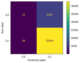
tn, fp, fn, tp = confusion_matrix(y_test, y_acc).ravel()
print("The precision of the model is: ", (tp/(tp+fp)))
print("The recall of the model is: ", (tp/(tp+fn)))
The precision of the model is:  0.8404041445435332
The recall of the model is:  0.998530042261285
OK so got a very good accuracy but it is still not good but why ?? There is a class imbalance that is the amount of rows representing 0 are much less as compared to the class 1
K = pd.concat([X, pd.Series(Y)], axis=1)
K.rename(columns={K.columns[-1]:"runs_off_bat"}, inplace=True)
# class count
class_count_1, class_count_0 = K["runs_off_bat"].value_counts()

# Separate class
class_0 = K[K['runs_off_bat'] == 0]
class_1 = K[K['runs_off_bat'] == 1]

# print the shape of the class
print('class 0:', class_0.shape)
print('class 1:', class_1.shape)
class 0: (31044, 9)
class 1: (163310, 9)
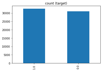
1. Random Under-Sampling (Method 1 of Dealing with Class Imbalance)
Undersampling can be defined as removing some observations of the majority class. This is done until the majority and minority classes have balanced out.
Undersampling can be a good choice when you have a ton of data. But a drawback to undersampling is that we are removing information that may be valuable.
class_1_under = class_1.sample(frac=0.2)

test_under = pd.concat([class_1_under, class_0], axis=0)

print("total class of 1 and 0:",test_under['runs_off_bat'].value_counts())# plot the count after under-sampeling
test_under['runs_off_bat'].value_counts().plot(kind='bar', title='count (target)')
total class of 1 and 0: 1.0    32662
0.0    31044
Name: runs_off_bat, dtype: int64


<AxesSubplot:title={'center':'count (target)'}>
X, Y = test_under.drop("runs_off_bat", axis=1), test_under["runs_off_bat"]
Lets again re-build our model using the new balanced dataset and see what is the output
X_train, X_test, y_train, y_test = train_test_split(X, Y, test_size=0.2)
model = xgb.XGBClassifier()
model.fit(X_train, y_train)
[21:22:04] WARNING: ../src/learner.cc:1115: Starting in XGBoost 1.3.0, the default evaluation metric used with the objective 'binary:logistic' was changed from 'error' to 'logloss'. Explicitly set eval_metric if you'd like to restore the old behavior.


XGBClassifier(base_score=0.5, booster='gbtree', colsample_bylevel=1,
              colsample_bynode=1, colsample_bytree=1, enable_categorical=False,
              gamma=0, gpu_id=-1, importance_type=None,
              interaction_constraints='', learning_rate=0.300000012,
              max_delta_step=0, max_depth=6, min_child_weight=1, missing=nan,
              monotone_constraints='()', n_estimators=100, n_jobs=4,
              num_parallel_tree=1, predictor='auto', random_state=0,
              reg_alpha=0, reg_lambda=1, scale_pos_weight=1, subsample=1,
              tree_method='exact', validate_parameters=1, verbosity=None)
y_acc = model.predict(X_test)
print("The % Accuracy of the Model is: ", accuracy_score(y_test, y_acc) * 100)
The % Accuracy of the Model is: 55.68984460838173
plot_confusion_matrix(model, X_test, y_test)
<sklearn.metrics._plot.confusion_matrix.ConfusionMatrixDisplay at 0x7f85623acf70>

tn, fp, fn, tp = confusion_matrix(y_test, y_acc).ravel()

print("The precision of the model is: ", (tp/(tp+fp)))
print("The recall of the model is: ", (tp/(tp+fn)))
The precision of the model is:  0.5677182685253118
The recall of the model is:  0.5889785355457452
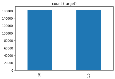
2. Random Over-Sampling
Oversampling can be defined as adding more copies to the minority class. Oversampling can be a good choice when you don’t have a ton of data to work with.
A con to consider when undersampling is that it can cause overfitting and poor generalization to your test set.
class_0_over = class_0.sample(class_count_1, replace=True)

test_over = pd.concat([class_0_over, class_1], axis=0)

print("total class of 1 and 0:",test_over['runs_off_bat'].value_counts())# plot the count after under-sampeling
test_over['runs_off_bat'].value_counts().plot(kind='bar', title='count (target)')
total class of 1 and 0: 0.0    163310
1.0    163310
Name: runs_off_bat, dtype: int64


<AxesSubplot:title={'center':'count (target)'}>
X, Y = test_over.drop("runs_off_bat", axis=1), test_over["runs_off_bat"]
X_train, X_test, y_train, y_test = train_test_split(X, Y, test_size=0.2)
model = xgb.XGBClassifier()
model.fit(X_train, y_train)
[21:23:39] WARNING: ../src/learner.cc:1115: Starting in XGBoost 1.3.0, the default evaluation metric used with the objective 'binary:logistic' was changed from 'error' to 'logloss'. Explicitly set eval_metric if you'd like to restore the old behavior.


XGBClassifier(base_score=0.5, booster='gbtree', colsample_bylevel=1,
              colsample_bynode=1, colsample_bytree=1, enable_categorical=False,
              gamma=0, gpu_id=-1, importance_type=None,
              interaction_constraints='', learning_rate=0.300000012,
              max_delta_step=0, max_depth=6, min_child_weight=1, missing=nan,
              monotone_constraints='()', n_estimators=100, n_jobs=4,
              num_parallel_tree=1, predictor='auto', random_state=0,
              reg_alpha=0, reg_lambda=1, scale_pos_weight=1, subsample=1,
              tree_method='exact', validate_parameters=1, verbosity=None)
y_acc = model.predict(X_test)
print("The % Accuracy of the Model is: ", accuracy_score(y_test, y_acc) * 100)
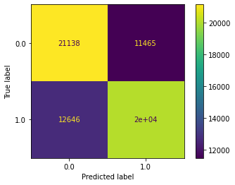
The % Accuracy of the Model is: 63.09013532545465
plot_confusion_matrix(model, X_test, y_test)
<sklearn.metrics._plot.confusion_matrix.ConfusionMatrixDisplay at 0x7f85cec10700>
tn, fp, fn, tp = confusion_matrix(y_test, y_acc).ravel()

print("The precision of the model is: ", (tp/(tp+fp)))
print("The recall of the model is: ", (tp/(tp+fn)))
The precision of the model is:  0.6364933417882055
The recall of the model is:  0.6135203691818709
Conclusions
- Got an Accuracy of 45% using Multi-Class Classification
- Got an Accuracy of 84 using Binary Classification , (predicting 1 for runs b/w 0–3 and 0 for runs >=4)
- Fixing class imbalance we get an accuracy of :
- 56 % on Under-Sampling Techniques
- 64% on Over-Sampling Techniques
So that’s it that was all about IPL Prediction , I hope you liked this post , if you did please let me know in the comments and if you want me to improve then also please let me know what should I emphasise on , I’ll definitely try my best .
Thank you geeks, see ya !!
Notebook available at : https://www.kaggle.com/code/neelakashchatterjee/ipl-per-ball-analysis-and-prediction

